Free Askey--Wilson functionals and geometric last passage percolation on a strip

Jacek Wesolowski; Kamil Szpojankowski; Wlodek Bryc

REVIEW 3 major objections 4 minor 12 references

Free Askey--Wilson functionals and geometric last passage percolation on a strip

T0 review · 3 major / 4 minor · reviewed 2026-08-07 · deepseek-v4-flash

Challenge this review Re-run · record.json Download PDF Read on arXiv ↗

Pith's one-line read A single functional identity gives the full phase diagram of geometric LPP on a strip.

desk verdict The phase diagram result is real and the main proofs hold up, but Proposition 2.15(iii) and equations (3.21)-(3.22) contain typos that need correction before the paper is publishable. read the letter →

arxiv 2506.01879 v1 pith:ARZGJJOH submitted 2025-06-02 math.PR

Wlodek Bryc , Kamil Szpojankowski , Jacek Wesolowski This is my paper

classification math.PR MSC 60K3533D4582B23

keywords geometriclastpassagepercolationstationarymeasurefreeAskey-WilsonfunctionalspolynomialsphasediagramPoissonapproximationstripq=0

verification ladder T0 review T1 audit T2 compute T3 formal

The pith

A machine-rendered reading of the paper's core claim, the machinery that carries it, and where it could break.

The reading

This paper establishes a representation for the multipoint generating function of geometric last passage percolation (LPP) on a finite-width strip: the generating function equals an iterated free Askey-Wilson functional, a $q=0$ relative of the classical Askey-Wilson moment functional. The representation holds for boundary parameters over a wider range than previous contour-integral formulas, and from it the authors read off the full phase diagram for the large-scale limit of $L_1(N)/N$, the height of the last passage line at the left end of the strip. In the bulk regime the limit is $a/(1-a)$; in two boundary-dominated regimes the limits are $a/(c_1-a)$ and $ac_2/(1-ac_2)$; and on the critical diagonal $c_1=c_2=c>1$ the limit is a random uniform mixture of the two boundary values. The paper also proves a Poisson approximation for the line profile when the boundary parameters vary with strip width. If the main identity holds, it provides a single analytic object governing the stationary measure's large-scale behaviour.

What carries the argument

The key object is the free Askey-Wilson functional $L^{(a,b,c)}$, the $q=0$ specialization of the Askey-Wilson moment functional: a linear functional on analytic functions defined by contour integration on ellipses $z=w+1/w$ with kernel $(1-w^2)(1-abcw)/(w(1-aw)(1-bw)(1-cw))$, which reduces to integration against signed measures when the parameters are small enough. Composition is handled by letting two parameters depend on a variable through $u(x)$, the Joukowsky inverse, producing functionals $\pi_{t;c_2}=L^{(c_2t,c_1/t)}$ and $P^{s,t;c_2}_x=L^{(c_2t,su(x)/t,s/(tu(x)))}$. The reduction formula $L^{(a,b,c)}[h_c f]=(1-ac)(1-bc)L^{(a,b)}[f]$ and its variant Corollary 2.14 replace the parameter $c_2$ by $a$ up to a multiplicative factor, and this change-of-parameter identity drives the induction proving Theorem 1.4. The accompanying asymptotic expansions of $L^{(a,b,c)}[h_v^{-n}]$ as $n\to\infty$, with simple-pole, double-pole and boundary cases, supply the exponential rates and prefactors whose ratios give the four limiting densities in Theorem 1.3.

What would settle it

Take fixed $c_1=c_2=c\in(1,1/a)$ and compute the normalization $Z_N=G_N(1)$ for large $N$ from the exact sum (1.3). The claim (3.21) predicts $Z_N\sim \frac{(c^2-1)^2}{a c^2(c-a)(1-ac)}\,N\,\left(\frac{c}{(c-a)(1-ac)}\right)^N$. A numerical check of the ratio $Z_N N^{-1}\left(\frac{(c-a)(1-ac)}{c}\right)^N$ against this constant, or a direct comparison of the two-atom Laplace transform (3.22) with the uniform-mixture formula, would settle whether the central phase-diagram claim is right.

Watch

Extended reading notes

Core claim

The paper's central claim is Theorem 1.4: for $0<a<1$, $ac_1<1$, $0<t_1\le\cdots\le t_N$ with $at_N<1$ and $a t_N^2 c_2<1$, the $N$-point generating function of the stationary measure satisfies $G_N^{(a,c_1,c_2)}(t)=\pi_{t_1,\ldots,t_N;c_2}[\bigotimes_{j=1}^N 1/h_{a t_j}]$, where $\pi$ is the composition of free Askey-Wilson functionals defined through the inverse Joukowsky map. The authors prove this identity by induction using a recurrence for the generating function and a matching recurrence for the functionals, without invoking the earlier contour-integral derivation. From the identity they obtain the Laplace transform of $L_1(N)/N$ as a ratio of two evaluations of the same functional, and asymptotic expansions of those evaluations yield the phase diagram of Theorem 1.3 and the Poisson convergence of Theorem 1.5.

Load-bearing premise

The phase diagram is read off from asymptotic expansions of $L^{(a,b,c)}[h_v^{-n}]$ (formulas (2.51)-(2.54)); if any of those expansions has a wrong constant or pole order — the double-pole case (2.53) is stated with details omitted — the limiting densities and the uniform mixture on the diagonal would be different.

Editorial extensions

If this is right

If $c_1,c_2\le 1$, then $L_1(N)/N\to a/(1-a)$ in probability, independent of the boundary parameters.
If $c_1>1$ and $c_2<c_1<1/a$, the limit becomes $a/(c_1-a)$, set by the left boundary.
If $c_2>1$ and $c_1<c_2<1/a$, the limit becomes $ac_2/(1-ac_2)$, set by the right boundary.
On the diagonal $c_1=c_2=c\in(1,1/a)$, the limit law is the uniform mixture $(a/(c-a))U+(ac/(1-ac))(1-U)$ with $U\sim\mathrm{Unif}[0,1]$.
Under two scalings of the parameters with strip width $N$, the process $(L_1(\lfloor Nx\rfloor))_{0\le x\le 1}$ converges in finite-dimensional distributions to a Poisson process of rate $\lambda$.

Reading between the lines

Editorial extensions of the paper, not claims the author makes directly.

The same functional calculus should apply to other $q=0$ integrable models; for the six-vertex model on a strip, where a similar phase diagram has been reported, the free Askey-Wilson composition could yield an equally explicit proof of the limiting regimes.
The signed-measure representations in Appendix B suggest that fluctuation exponents in the boundary-dominated regimes can be extracted from the atomic parts of the measures, in analogy with ASEP shock fluctuations; the paper does not compute such fluctuations.
A testable extension is to replace the Laplace-transform convergence criterion by a direct steepest-descent analysis of the contour integrals in Proposition 2.12, which would sharpen error terms in Theorem 1.3 and possibly reveal the $N^{1/3}$ scale.
The Poisson theorem suggests that when $a$ and $c_2$ are tuned as $N\to\infty$, the strip becomes effectively one-dimensional at the left boundary; this may be the first member of a family of Poisson-type limits for multi-layer polymers on strips.

Share X Bluesky LinkedIn Reddit HN

Editorial analysis

A structured set of objections, weighed in public.

Desk editor's note, referee report, and a circularity audit.

Desk Editor's Note

read the letter

The paper does what it claims: it introduces free Askey-Wilson functionals, proves Theorem 1.4 (the multipoint generating function representation) by a self-contained recurrence induction, and derives the phase diagram (Theorem 1.3) plus a Poisson limit (Theorem 1.5). The novelty is solid: the formulas work for a wider boundary-parameter range than Barraquand's contour integrals, and the phase diagram was predicted by universality but not previously derived for this model. The authors give credit where due and the proof strategy is independent of Barraquand's contour formulas, which is good.

The main soft spot is a string of typos in the asymptotic expansions that support the diagonal case c1=c2=c>1. Proposition 2.15(iii) as printed is false: (2.53) states L ~ C(a,c) v^n [a/((a-v)(1-av))]^{n+1}, but the proof in Section 2.6 derives a double-pole residue that gives C(a,c) * n * v * [a/(...)]^{n+1}. The printed version lacks the factor n and has v^n instead of v. This is not cosmetic: Theorem 1.3(iv) and the normalization Z_N in (3.21) depend on this. I also found (3.21) itself is off by a factor a^2: it should be (c^2-1)^2 a N c^{N-2}/((c-a)(1-ac))^{N+1}, not with 1/a in the denominator. Similarly, the second atom term in (3.22) should have (c-a t_N^2)^N, not (c-a t_N)^N. Recomputing the Laplace transform ratio with these corrections gives exactly the mixture in (1.10), so the theorem is right; the printed equations are not. A referee should ask for these to be fixed, and also for the omitted boundary cases c1=1 or c2=1 in Theorem 1.3(i).

The rest of the paper is in better shape. The recurrence-based proof of Theorem 1.4 is detailed and the appendix computations are thorough. The asymptotic machinery in Proposition 2.15(i),(ii),(iv) also checks out. The Poisson theorem is technically involved and I did not find an error there, though I did not re-derive every step.

Who is this for: people working in integrable probability and exact solvability, especially those interested in stationary measures of polymer models. It deserves a serious referee because the main results are significant and the proofs are largely sound once the typos are repaired. I would not desk-reject.

In short: engage with it, send it to referees, but tell the authors to fix the asymptotic formulas and complete the boundary-case proof.

Referee Report

3 major / 4 minor

Summary. The paper introduces free Askey-Wilson functionals L^{(a,b,c)} and uses them to give a multipoint generating function for geometric last passage percolation on a strip, stated as Theorem 1.4. The proof is an induction based on recurrences (3.1) and (3.3), with detailed appendix computations, and does not rely on Barraquand's contour integral formulas. From this representation the authors derive the phase diagram for the large-N limit of L_1(N)/N, Theorem 1.3, including the random uniform mixture on the diagonal, and a Poisson approximation under varying parameters, Theorem 1.5. The Laplace-transform asymptotics in Section 2.6 are the mechanism that turns the generating-function identity into the phase diagram.

Significance. If the asymptotic results are correct, the paper settles the phase diagram for the stationary measure of geometric LPP on a strip and adds a Poisson approximation, giving a substantial extension of the accessible boundary-parameter range. The free Askey-Wilson functional framework is a new tool in this context. A notable strength is that Theorem 1.4 is proved self-contained from recurrences, with the phase-diagram constants derived rather than fitted. The main weakness is the current state of Proposition 2.15(iii), whose printed asymptotic is inconsistent with its own proof; since Theorem 1.3(iv) rests on that asymptotic, the proof is not complete as written.

major comments (3)

[2.6, Eq. (2.53)] The double-pole asymptotic in (2.53) is inconsistent with its proof. In the proof of (2.53), the residue calculation gives L^{(a,b,c)}[h_v^{-n}] ~ n z_a^{-(n+1)} Psi(z_a), with Psi(z_a) = (a^2-1)^2 v(1-ac)/(a^2(a-c)) and z_a^{-1} = a/((a-v)(1-av)). This yields C(a,c) n v [a/((a-v)(1-av))]^{n+1}, not C(a,c) v^n [a/((a-v)(1-av))]^{n+1}. The printed formula has v^n where the proof gives n v. This is load-bearing: Theorem 1.3(iv) uses (2.53) to obtain the normalization Z_N in (3.21), and (3.23) uses that normalization to produce the uniform mixture in (1.10). As printed, (2.53) is false; for example, at v=a and c=0 it has a^N where the corrected asymptotic has N. The formula and the resulting constants in (3.21) and (3.23) must be corrected and rechecked before the phase-diagram proof is complete.
[3.3.1, Theorem 1.3(i)] Theorem 1.3(i) is stated for c1,c2 <= 1, but the proof in Section 3.3.1 explicitly assumes c1,c2 < 1 and says 'the argument need to be modified and is omitted' for the boundary. Since c1 = 1 or c2 = 1 belongs to the statement of the theorem, this is a gap in the proof of the full phase diagram. Please either supply the boundary argument, for example using (2.54) after completing its proof, or restrict the statement of Theorem 1.3(i) to the open region and state the boundary cases separately.
[2.6, proof of (2.54)] The proof of (2.54) contains the sentence '(Here we omitted some details)' immediately after a dominated-convergence step, and the interchange of limit and integral is not fully justified. This asymptotic is needed for the boundary cases c = 1 in Theorem 1.3(i), which are currently omitted. As written, the proof of (2.54) is a sketch; please complete the justification, for instance by supplying a uniform integrability bound for the integrand after the change of variables u = (2-y)n.

minor comments (4)

[2.6, Eq. (2.53)] The notation in Proposition 2.15 uses a for a functional parameter that in Theorem 1.3 is also called a, leading to confusion when the proposition is applied with a = c and v = a. Consider using different letters in the proposition or explicitly stating the substitution in Section 3.3.4.
[3.3.4, Eq. (3.21)] After correcting (2.53), the displayed normalization in (3.21) still appears to have a misprint: substituting the corrected (2.53) with functional parameters c,c,0 and v=a gives a factor a in the numerator of the prefactor, not in the denominator. The subsequent line (3.23) appears consistent with the corrected normalization, so this is likely a typographical error, but it should be fixed.
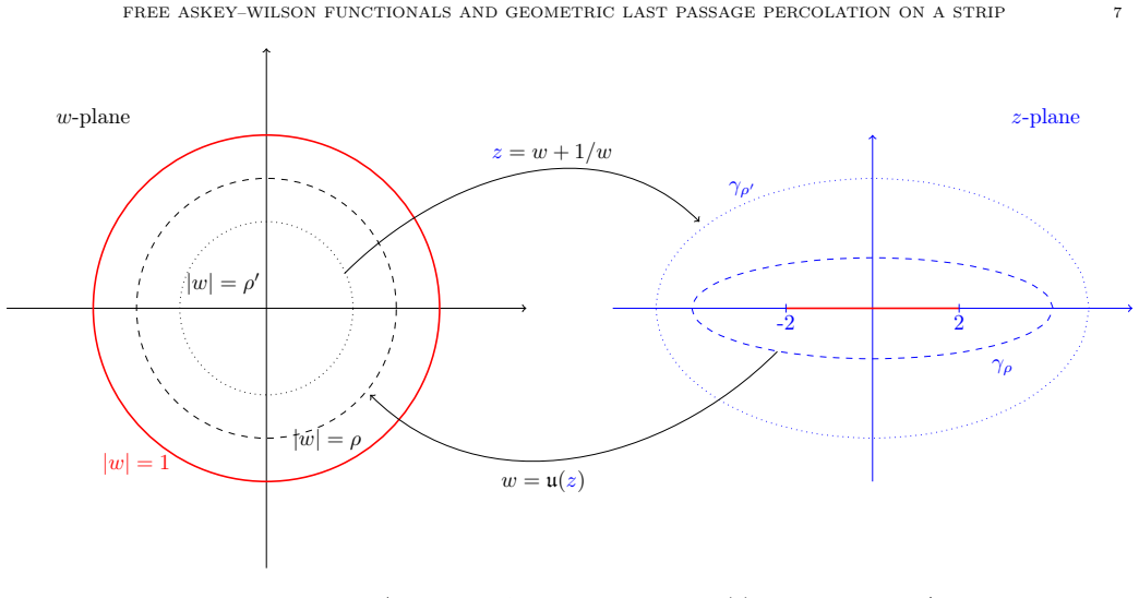
[2.3.1, Fig. 2] The text says the ellipse gamma_rho in (2.22) is oriented clockwise, while later integrals are taken counter-clockwise. This is presumably intentional and resolved by the 'standard convention' sentence, but the figure caption and (2.22) could be clarified to avoid confusion.
[3.3, final paragraph] The use of [Mukherjea et al., 2006, Theorem 2] to pass from Laplace-transform convergence to weak convergence is terse; please state the exact theorem or give a self-contained argument, especially because the limiting formulas in Theorem 1.3 involve a random mixture rather than a deterministic limit.

Circularity Check

0 steps flagged · score 0.0 of 10

No circularity: Theorem 1.4 is proved by recurrence from the original two-layer ensemble, and the phase-diagram limits are obtained from computed asymptotics, not fitted inputs.

full rationale

The central derivation chain is self-contained. Theorem 1.4 is proved by induction from the explicit recurrences (3.1) (proved in Appendix A from the sum over the two-layer ensemble) and (3.3) (proved from the reduction formula (2.49)), with the base case computed directly from the geometric series; the proof does not rely on Barraquand's contour formulas, which are cited only as inspiration. The phase diagram (Theorem 1.3) is then obtained by substituting t=e^{s/N} into (1.15) and estimating the Laplace transform via the asymptotic expansions (2.51)-(2.54); the limiting densities a/(1-a), a/(c1-a), ac2/(1-ac2), and the uniform mixture on the diagonal are read off exponential rates and residues, not fitted to data. Theorem 1.5 is likewise an analytic application of the same representation rather than a prediction from fitted constants. The prior works of the same authors that are cited (Szpojankowski 2010, Wang-Wesolowski-Yang 2024, Bryc-Wesolowski 2017) are either reproved in the present text, used as context, or appear in notation remarks; they are not load-bearing and therefore do not constitute circularity. I additionally flag, as a correctness concern rather than circularity, that Proposition 2.15(iii) as printed appears internally inconsistent: the residue computation in its proof gives an asymptotic with a factor n v (matching the later use in (3.21)), while displayed equation (2.53) has v^n; this should be corrected but does not affect the circularity assessment.

Assumptions & free parameters 0 free parameters · 2 assumptions · 1 invented entities

The model's stationary measure is imported from Barraquand-Corwin-Yang; the asymptotics machinery is derived in the paper. No parameters are fitted to data. The new functional is explicitly defined and verified on polynomials, so it is not an ad hoc entity.

assumptions (2)

domain assumption The unique stationary measure of geometric LPP on a strip is the marginal of the two-layer ensemble Q (Barraquand, Corwin, Yang).
Imported from Theorem 1.1; the paper uses this identification to translate asymptotics of L1(N) into statements about the stationary measure.
standard math Standard tools of complex analysis: Joukowsky map inverses, residue theorem, Mergelyan approximation, dominated convergence.
Used to define and extend the free Askey-Wilson functionals and to analyze their asymptotics.

invented entities (1)

Free Askey-Wilson functionals L^{(a,b,c)} independent evidence
purpose: Represent multipoint generating functions of the geometric LPP strip model as iterated functionals, extending Barraquand's contour integral formulas to the full parameter range.
Definition 2.2 gives an explicit contour integral and Proposition 2.3 verifies agreement with the free Askey-Wilson polynomial moment functional; these properties are checkable independently of the LPP application.

how reviews work

0 comments

Cite this review

Pith. "Pith review of Free Askey--Wilson functionals and geometric last passage percolation on a strip." pith.science (2026). https://pith.science/paper/ARZGJJOH

@misc{pith2026250601879,
  author       = {Pith},
  title        = {Pith review of: Free Askey--Wilson functionals and geometric last passage percolation on a strip},
  year         = {2026},
  howpublished = {\url{https://pith.science/paper/ARZGJJOH}},
  note         = {Machine review of arXiv:2506.01879}
}

abstract

Barraquand, Corwin, and Yang arXiv:2306.05983 established that geometric last passage percolation (LPP) on a strip of $\mathbb{Z}^2$ has a unique stationary measure. Building on this, Barraquand arXiv:2409.08927 derived explicit contour integral formulas for the model's multipoint probability generating function. In this paper, we introduce free Askey--Wilson functionals and use them to extend these generating function formulas. Our framework yields explicit expressions valid over a broader range of boundary parameters than previously accessible. This generalization allows us to determine the full phase diagram that characterizes how the large-scale asymptotics of the stationary measure depend on the boundary conditions. In addition, we prove a Poisson approximation for the stationary measure when the parameters vary with the strip width.

Figures

Figures reproduced from arXiv: 2506.01879 by the authors.

**Figure 1.** The limit 1 N L1(N) → ρ = ρ(a, c1, c2) and the boundary parameters c1, c2 ∈ (0, 1/a). Below the hyperbola c1c2 = 1, the functional π t in (1.12) is given as an integral with respect to a positive Askey–Wilson measure. For (c1, c2) ∈ I := (0, 1]2 the limit does not depend on the boundary parameters. The line between the points (1,1) and (1/a, 1/a) separates the regions L and H with the low and high average and the li… view at source ↗

**Figure 2.** Mapping z = w + 1/w and one of its two inverses w = u(z). Note that with ρ ′ < ρ, ellipse γρ lies inside γρ′ . maps injectively C \ [−2, 2] onto the unit disk |w| < 1. We extend u to z ∈ [−2, 2] by taking u(x) = e iθ for x = 2 cos θ with 0 ≤ θ ≤ π. Then u is the right inverse of the Joukowsky map: u(z) + 1 u(z) = z for all z ∈ C. The second inverse mapping, 1/u(z) = (z + √ z 2 − 4)/2 maps injectively C \ [−2, 2] ont… view at source ↗

Discussion (0). Sign in to comment.

Reference graph

Works this paper leans on

12 extracted references · 11 canonical work pages

[1]

Ahlfors, L. V. (1978). Complex analysis . International Series in Pure and Applied Mathematics. McGraw-Hill Book Co., New York, third edition

work page 1978
[2]

and Wilson, J

Askey, R. and Wilson, J. (1985). Some basic hypergeometric orthogonal polynomials that generalize J acobi polynomials. Mem. Amer. Math. Soc. , 54(319):iv+55

work page 1985
[3]

Barraquand, G. (2024). Integral formulas for two-layer S chur and W hittaker processes. https://arxiv.org/abs/2409.08927

arXiv 2024
[4]

Barraquand, G., Corwin, I., and Yang, Z. (2024). Stationary measures for integrable polymers on a strip. Invent. Math. , 237(3):1567--1641

work page 2024
[5]

Asymmetric Simple Exclusion Process with open boundaries and Quadratic Harnesses

Bryc, W. and Weso owski, J. (2017). Asymmetric simple exclusion process with open boundaries and quadratic harnesses. J. Stat. Phys. , 167(2):383--415. https://arxiv.org/abs/1511.01163

work page Pith review arXiv 2017
[6]

R., Hakim, V., and Pasquier, V

Derrida, B., Evans, M. R., Hakim, V., and Pasquier, V. (1993). Exact solution of a 1 D asymmetric exclusion model using a matrix formulation. J. Phys. A , 26(7):1493--1517

work page 1993
[7]

Markushevich, A. I. (1977). Theory of functions of a complex variable. V ol. I , II , III . Chelsea Publishing Co., New York, english edition

work page 1977
[8]

Mukherjea, A., Rao, M., and Suen, S. (2006). A note on moment generating functions. Statist. Probab. Lett. , 76(11):1185--1189

work page 2006

Show all 12 references

[9]

Rudin, W. (1987). Real and complex analysis . McGraw-Hill Book Co., New York, third edition

1987
[10]

Szpojankowski, K. (2010). Free quadratic harnesses. Master's thesis, (2010) Warsaw Univ. Techn. (in Polish)

2010
[11]

Wang, Y., Weso owski, J., and Yang, Z. (2024). Askey- W ilson signed measures and open ASEP in the shock region. Int. Math. Res. Not. IMRN , (15):11104--11134. https://arxiv.org/pdf/2307.06574

2024 arXiv
[12]

Yang, Z. (2024). Stationary measure for six-vertex model on a strip. Electron. J. Probab. , 29:Paper No. 44, 28

2024

Pith tools

Reviewed August 7, 2026 · model on record in the stance chip above.

[1] [1]

Ahlfors, L. V. (1978). Complex analysis . International Series in Pure and Applied Mathematics. McGraw-Hill Book Co., New York, third edition

work page 1978

[2] [2]

and Wilson, J

Askey, R. and Wilson, J. (1985). Some basic hypergeometric orthogonal polynomials that generalize J acobi polynomials. Mem. Amer. Math. Soc. , 54(319):iv+55

work page 1985

[3] [3]

Barraquand, G. (2024). Integral formulas for two-layer S chur and W hittaker processes. https://arxiv.org/abs/2409.08927

arXiv 2024

[4] [4]

Barraquand, G., Corwin, I., and Yang, Z. (2024). Stationary measures for integrable polymers on a strip. Invent. Math. , 237(3):1567--1641

work page 2024

[5] [5]

Asymmetric Simple Exclusion Process with open boundaries and Quadratic Harnesses

Bryc, W. and Weso owski, J. (2017). Asymmetric simple exclusion process with open boundaries and quadratic harnesses. J. Stat. Phys. , 167(2):383--415. https://arxiv.org/abs/1511.01163

work page Pith review arXiv 2017

[6] [6]

R., Hakim, V., and Pasquier, V

Derrida, B., Evans, M. R., Hakim, V., and Pasquier, V. (1993). Exact solution of a 1 D asymmetric exclusion model using a matrix formulation. J. Phys. A , 26(7):1493--1517

work page 1993

[7] [7]

Markushevich, A. I. (1977). Theory of functions of a complex variable. V ol. I , II , III . Chelsea Publishing Co., New York, english edition

work page 1977

[8] [8]

Mukherjea, A., Rao, M., and Suen, S. (2006). A note on moment generating functions. Statist. Probab. Lett. , 76(11):1185--1189

work page 2006