REVIEW 4 major objections 6 minor 40 references
Localized Functional Principal Component Analysis Based on Covariance Structure
T0 review · 4 major / 6 minor · reviewed 2026-08-07 · deepseek-v4-flash
Pith's one-line read This paper shows that if a process splits into uncorrelated sub-processes on disjoint intervals, applying FPCA to each piece yields eigenfunctions of the whole process that are automatically localized and orthogonal.
desk verdict A clean, correct L-FPCA method for exactly block-diagonal covariances, but it does not yet face the near-block-diagonal case that real data will present. read the letter →
The pith
A machine-rendered reading of the paper's core claim, the machinery that carries it, and where it could break.
The reading
What carries the argument
The argument is carried by the block-diagonal covariance structure, the Karhunen-Loève expansion of each sub-process, and BD-SVD, a singular-vector-based algorithm that detects the block-diagonal covariance structure from the noisy sample covariance. Lemma 1 ties zero cross-block covariance to compactly supported sub-process eigenfunctions, Lemma 2 equates sub-process eigenfunctions and eigenvalues with those of the full process on each interval, and Corollary 2 gives orthonormality of the assembled localized eigenfunctions.
What would settle it
Run L-FPCA on simulated curves with a known block-diagonal covariance: if the detected supports are wrong by more than a few grid points, or if the per-block PVE differs from the true block PVE by more than sampling variability, the pipeline fails. A sharper version adds a small constant $\varepsilon$ to off-block covariance entries and checks whether the estimated eigenfunctions leak outside their supports.
Extended reading notes
Core claim
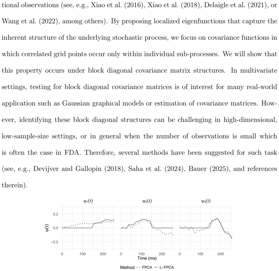
The central claim is Lemma 2: under the block-diagonal covariance assumption, the eigenfunctions and eigenvalues of each sub-process $X_k$ on its interval $T_k$ coincide with those of the full process $X$ on that interval. Corollary 1 then states that all eigenfunctions of $X$ are compactly supported on single intervals, so the sparse structure of the process is mirrored by the eigenfunctions without any explicit sparsity penalty. Consequently, Procedure 1 — detect blocks via a singular-vector block-detection algorithm, run FPCA on each block, sort the eigenvalues — directly produces orthonormal localized principal components.
Load-bearing premise
The construction assumes the covariance $\Gamma(s,t)$ is exactly zero whenever $s$ and $t$ lie in different intervals of the partition; if small cross-block correlations exist, the true eigenfunctions are not exactly zero outside their blocks and the hard block constraint will bias the estimated eigenfunctions and eigenvalues.
Editorial extensions
If this is right
- Because the localized eigenfunctions are orthonormal by construction, the explained variance of the full process is additive across sub-processes, so each interval's contribution can be read directly from its eigenvalues.
- The PVE of a sub-process equals the sum of its eigenvalues divided by the total variance, which follows from Lemma 2; this makes per-region explained variance available even when a region contributes multiple components.
- Since L-FPCA never penalizes the eigenfunctions, the estimated eigenvalues and PVEs do not suffer the over-regularization shrinkage observed for penalized sparse FPCA in the simulation study.
- The number of blocks detected by BD-SVD determines both the number of localized components and the partition of the domain, so the method outputs a domain segmentation alongside the principal components.
Reading between the lines
- Beyond the paper: the same block-diagonal reasoning should extend to multidimensional domains $T\subset\mathbb{R}^d$, where blocks become product regions, provided the cross-region covariance vanishes; the orthogonality argument would carry over unchanged.
- Beyond the paper: the hard zero-covariance assumption invites a natural stress test — simulate from an approximately block-diagonal covariance and measure how support recovery and per-block PVE degrade as off-block correlations grow.
- Beyond the paper: the EEG result that alcoholic and control groups differ in the number of detected sub-processes implies the block count itself could serve as a classification feature, a use the paper mentions only as a future direction.
Editorial analysis
A structured set of objections, weighed in public.
Referee Report
Summary. The paper proposes a localized functional principal component analysis (L-FPCA) method built on the assumption that the covariance function of the stochastic process is block-diagonal with respect to a partition of the domain. Under this assumption, the process decomposes into uncorrelated sub-processes on disjoint intervals, and the eigenfunctions of the full process coincide on each interval with the eigenfunctions of the corresponding sub-process. The proposed Procedure 1 detects the block structure via BD-SVD (Bauer 2025), then applies standard FPCA within each detected block, yielding localized eigenfunctions that are orthonormal by construction. The paper provides theoretical lemmas (Lemma 1, Lemma 2, Corollary 1, Corollary 2) establishing these equivalences, a simulation study comparing L-FPCA with thresholded FPCA and SFPCA, and two real-data applications (pinch force curves and EEG data).
Significance. If the block-diagonal assumption holds exactly, the method provides localized eigenfunctions that coincide with the population eigenfunctions on each block, avoiding the over-regularization and non-orthogonality issues of penalized approaches. The theoretical development is elementary but sound under assumption (3), and the simulation study is carefully designed to show the method's support-recovery and variance-explained performance in the exact block-diagonal setting. The paper ships reproducible R code and a detailed supplementary appendix, which is a strength. However, the practical relevance of the method is currently limited by the strength of the block-diagonal assumption and by the absence of any analysis of what happens when the covariance is only approximately block-diagonal, which is the realistic regime for functional data.
major comments (4)
- [Section 3, Eq. (3) and Procedure 1] The exactness of Lemma 2 and Corollary 1 relies entirely on the population-level assumption (3) that Γ(s,t)=0 for s and t in different blocks. The last paragraph of Section 3 correctly notes that the empirical covariance perturbs the block structure, but the manuscript gives no analysis of the effect of nonzero off-block entries. When off-block correlations are small but nonzero, the eigenvalues of block submatrices are not eigenvalues of the full covariance operator, and the hard support constraints imposed in Step 1 of Procedure 1 force estimated eigenfunctions to be exactly zero in regions where the true eigenfunctions are merely small. The simulation study in Section 4 generates data from exactly block-diagonal covariances in both designs, so this misspecification regime is never exercised. I request a concrete error analysis (e.g., bounds on eigenfunction and eigenvalue bias as a function of the operator norm of the off-block part of Γ) or, at minimum, a simulation that adds off-block correlations of varying magnitude and reports bias in eigenfunctions, eigenvalues, and support recovery.
- [Section 3, last paragraph; Procedure 1, Step 1] The method depends critically on BD-SVD (Bauer 2025) to recover the unknown blocks from finite noisy data, but no consistency theorem for BD-SVD in the functional setting is stated, and no result quantifies how detection errors propagate to the estimated localized eigenfunctions and eigenvalues. Because Step 1 is the only data-dependent step that determines the support of every eigenfunction, an incorrect block partition directly changes the output. Please add either a support-recovery consistency result (e.g., as N and the grid density grow, the estimated blocks converge to the true blocks with probability tending to one) or a sensitivity analysis that varies the signal-to-noise ratio and the separability of blocks in the simulation.
- [Section 4.2, Definition of Specificity and Precision] The text states that "TN denotes the number of correctly identified grid points in the support" and "TP the number of correctly identified grid points outside the support," but the formulas immediately below—TN=|S^c_hat∩S^c| and TP=|S_hat∩S|—define TN as correctly identified points outside the support and TP as correctly identified points inside the support. The labeling is reversed and makes the interpretation of Figure 2 ambiguous. Please correct the terminology or the formulas.
- [Section 5.2, EEG application] The real-data analysis interprets the intervals detected by BD-SVD as "uncorrelated sub-processes" and draws comparative conclusions about the number of blocks in the alcoholic versus control groups. The paper provides no diagnostic or test supporting the plausibility of the block-diagonal assumption (3) for these data; the observed difference in block counts could partly reflect different noise levels or signal complexity between groups rather than a genuine difference in the number of uncorrelated sub-processes. Please add a diagnostic of off-block correlation strength (e.g., a permutation-based summary of the empirical covariance outside the detected blocks) or soften the causal interpretation of the group comparison.
minor comments (6)
- [Section 3, Lemma 1] Lemma 1 is vacuous as stated: the eigenfunctions of the sub-process X_k are compactly supported on T_k by the definition in (2), regardless of whether the cross-block covariance is zero. The substantive statement is Lemma 2, which requires (3). Consider reformulating Lemma 1 as a remark to avoid giving the impression that (3) is needed for the trivial support property.
- [Section 4.1 and 4.2, threshold values] The threshold values for FPCA(τ) are inconsistent: Section 4.1 states τ=10^{-3} and τ=10^{-5}, while Section 4.2 and the caption of Figure 2 use 10^{-3} and 10^{-4}. Please align these values.
- [Section 4.1, M=10] The simulation uses 8 eigenvalues in the KL representation (8), but the text says "We pick M=10 eigenfunctions in all our scenarios." Clarify whether M=10 refers to the number of estimated components or the truncation level; the relationship between M and the 8 true components is not explained.
- [Procedure 1, Step 1] The text refers to "supports T_1,...,T_b" but the partition size is denoted K throughout the paper; this is a typo.
- [Section 4.3, equation reference] The text says "computing the percentage of variance explained (PVE) in (4.3)" but the displayed equation is not numbered; add a number or refer to the display directly.
- [Introduction, terminology] The phrase "uncorrelated sub-processes" is used as if it follows from the partition, but it is an assumption (3) about the covariance. Please make this explicit early in the paper to avoid confusion.
Circularity Check
No major circularity: the central block-diagonal spectral theorem is genuine, but Lemma 1's localization claim is partly built into the sub-process definition, and the practical block-detection step is delegated to a same-author citation.
-
self definitional
[Section 3, Lemma 1 (with Section 2, Eq. (2))]
"It holds that Γ(s, t) a.e. = 0 for s ̸∈ Tk and t ∈ Tk if and only if the eigenfunctions {ψk,j(·)}∞ j=1 of sub-process Xk(·) are compactly supported on Tk, namely ψk,j(t) = 0 for t /∈ Tk."
The sub-process Xk is defined in Eq. (2) to be exactly X(t) on Tk and 0 outside Tk. Therefore its covariance Γk(s,t) is identically zero whenever s or t is outside Tk, and any eigenfunction of Xk automatically vanishes outside Tk (for nonzero eigenvalue). This compact-support conclusion follows from the definition of Xk alone, not from the stated cross-block vanishing condition on Γ. Presenting Lemma 1 as an 'if and only if' consequence of the block structure makes localization look like an output when it is already an input of the decomposition. The genuinely nontrivial part, that these sub-process eigenpairs are also eigenpairs of X, is Lemma 2, which does depend on assumption (3) and is not circular.
full rationale
L-FPCA's central equivalence (Lemma 2 and Corollary 1) is a genuine spectral consequence of the block-diagonal covariance assumption (3): if Γ vanishes across disjoint intervals, the covariance operator splits into a direct sum, so the eigenpairs on each block are eigenpairs of the full operator. This derivation is self-contained and does not reduce to a fitted parameter or to a prediction that is forced by construction. The one step that is self-definitional is Lemma 1, because the sub-process Xk is defined to be zero outside Tk, so its eigenfunctions are automatically compactly supported on Tk regardless of the cross-block condition on Γ; the paper presents this as a derived 'if and only if' property, but the support is an input of the definition. The practical block-detection step is delegated to Bauer (2025), a same-author citation for BD-SVD; this is an external methodological dependency rather than a fitted parameter renamed as a prediction, and it does not make the theoretical claim circular. However, the paper supplies no consistency or misspecification analysis of BD-SVD in the functional setting, and the simulations generate data from exactly the block-diagonal model that BD-SVD is designed to recover, so the misspecified regime is never exercised. These are robustness concerns, not circularity. Overall score 2 reflects the minor self-definitional support claim, not the main spectral result.
Assumptions & free parameters
free parameters (1)
- Number of sub-processes K and partition boundaries
assumptions (3)
- domain assumption The covariance function Γ(s,t) is block diagonal with respect to the partition T1,...,TK, i.e., Γ(s,t)=0 for s in Ti, t in Tj, i≠j (equation (3)).
- standard math The stochastic process X is mean-zero, continuous, and square-integrable on a compact interval T, and its eigenelements have positive eigenvalues.
- ad hoc to paper The finite-dimensional truncation and the empirical covariance estimate preserve the block structure of the true covariance, and BD-SVD recovers this structure correctly.
Cite this review
Pith. "Pith review of Localized Functional Principal Component Analysis Based on Covariance Structure." pith.science (2026). https://pith.science/paper/RYVG24HN
@misc{pith2026250602836,
  author       = {Pith},
  title        = {Pith review of: Localized Functional Principal Component Analysis Based on Covariance Structure},
  year         = {2026},
  howpublished = {\url{https://pith.science/paper/RYVG24HN}},
  note         = {Machine review of arXiv:2506.02836}
}
read the original abstract
Functional principal component analysis (FPCA) is a widely used technique in functional data analysis for identifying the primary sources of variation in a sample of random curves. The eigenfunctions obtained from standard FPCA typically have non-zero support across the entire domain. In applications, however, it is often desirable to analyze eigenfunctions that are non-zero only on specific portions of the original domain-and exhibit zero regions when little is contributed to a specific direction of variability-allowing for easier interpretability. Our method identifies sparse characteristics of the underlying stochastic process and derives localized eigenfunctions by mirroring these characteristics without explicitly enforcing sparsity. Specifically, we decompose the stochastic process into uncorrelated sub-processes, each supported on disjoint intervals. Applying FPCA to these sub-processes yields localized eigenfunctions that are naturally orthogonal. In contrast, approaches that enforce localization through penalization must additionally impose orthogonality. Moreover, these approaches can suffer from over-regularization, resulting in eigenfunctions and eigenvalues that deviate from the inherent structure of their population counterparts, potentially misrepresenting data characteristics. Our approach avoids these issues by preserving the inherent structure of the data. Moreover, since the sub-processes have disjoint supports, the eigenvalues associated to the localized eigenfunctions allow for assessing the importance of each sub-processes in terms of its contribution to the total explained variance. We illustrate the effectiveness of our method through simulations and real data applications. Supplementary material for this article is available online.
Figures


Figures from the paper (3 more)


Reference graph
Works this paper leans on
-
[1]
Bauer, J. O. (2025). High-dimensional block diagonal covariance structure detection using singular vectors. J. Comput. Graph. Stat.\/ 0\/ (0), 1--12
work page 2025
-
[2]
Bauer, J. O. and B. Drabant (2021). Principal loading analysis . J. Multivar. Anal.\/ 184
work page 2021
-
[3]
Beyaztas, U., H. L. Shang, and A.-S. G. Abdel-Salam (2022). Functional linear models for interval-valued data. Commun. Stat. - Simul. Comput.\/ 51\/ (7), 3513--3532
work page 2022
-
[4]
Blanquero, R., E. Carrizosa, A. Jim \'e nez-Cordero, and B. Mart \' n-Barrag \'a n (2020). Selection of time instants and intervals with support vector regression for multivariate functional data. Comput. Oper. Res\/ 123 , 105050
work page 2020
-
[5]
Blanquero, R., E. Carrizosa, C. Molero-R \' o, and D. R. Morales (2023). On optimal regression trees to detect critical intervals for multivariate functional data. Comput. Oper. Res\/ 152 , 106152
work page 2023
-
[6]
Chen, K. and J. Lei (2015). Localized functional principal component analysis. J. Am. Stat. Assoc.\/ 110\/ (511), 1266--1275
work page 2015
-
[7]
Crainiceanu, C. M., J. Goldsmith, A. Leroux, and E. Cui (2024). Functional data analysis with R . CRC Press
work page 2024
-
[8]
Delaigle, A., P. Hall, W. Huang, and A. Kneip (2021). Estimating the covariance of fragmented and other related types of functional data. J. Am. Stat. Assoc.\/ 116\/ (535), 1383--1401
work page 2021
Show all 40 references
-
[9]
Hall, and T
Delaigle, A., P. Hall, and T. Pham (2019). Clustering functional data into groups by using projections. J. R. Stat. Soc. B\/ 81\/ (2), 271--304
2019
-
[10]
Devijver, E. and M. Gallopin (2018). Block-diagonal covariance selection for high-dimensional gaussian graphical models. J. Am. Stat. Assoc.\/ 113\/ (521), 306--314
2018
-
[11]
Di, C.-Z., C. M. Crainiceanu, B. S. Caffo, and N. M. Punjabi (2009). Multilevel functional principal component analysis. Ann. Appl. Stat.\/ 3\/ (1), 458
2009
-
[12]
Fan, J. and R. Li (2001). Variable selection via nonconcave penalized likelihood and its oracle properties. J. Am. Stat. Assoc.\/ 96\/ (456), 1348--1360
2001
-
[13]
Greven, and C
Goldsmith, J., S. Greven, and C. Crainiceanu (2013). Corrected confidence bands for functional data using principal components. Biometrics\/ 69\/ (1), 41--51
2013
-
[14]
M \"u ller, and J.-L
Hall, P., H.-G. M \"u ller, and J.-L. Wang (2006). Properties of principal component methods for functional and longitudinal data analysis . Ann. Stat.\/ 34\/ (3), 1493--1517
2006
-
[15]
Ieva, F., A. M. Paganoni, and N. Tarabelloni (2016). Covariance-based clustering in multivariate and functional data analysis. J. Mach. Learn. Res.\/ 17\/ (143), 1--21
2016
-
[16]
James, G. M. and C. A. Sugar (2003). Clustering for sparsely sampled functional data. J. Am. Stat. Assoc.\/ 98\/ (462), 397--408
2003
-
[17]
Xiao, and S
Li, C., L. Xiao, and S. Luo (2020). Fast covariance estimation for multivariate sparse functional data. Stat\/ 9\/ (1), e245
2020
-
[18]
Wang, and J
Lin, Z., L. Wang, and J. Cao (2016). Interpretable functional principal component analysis. Biometrics\/ 72\/ (3), 846--854
2016
-
[19]
Nie, Y. and J. Cao (2020). Sparse functional principal component analysis in a new regression framework. Comput. Stat. Data Anal.\/ 152 , 107016
2020
-
[20]
Pini, A. and S. Vantini (2016). The interval testing procedure: a general framework for inference in functional data analysis. Biometrics\/ 72\/ (3), 835--845
2016
-
[21]
Pini, A. and S. Vantini (2017). Interval-wise testing for functional data. J. Nonparametric Stat.\/ 29\/ (2), 407--424
2017
-
[22]
R: A Language and Environment for Statistical Computing
R Core Team (2022). R: A Language and Environment for Statistical Computing . Vienna, Austria: R Foundation for Statistical Computing
2022
-
[23]
Ramsay, J. (2024). fda: Functional Data Analysis . R package version 6.2.0
2024
-
[24]
Ramsay, J. and B. Silverman (2005). Functional Data Analysis . Springer Series in Statistics. Springer
2005
-
[25]
Rice, J. A. and B. W. Silverman (1991). Estimating the mean and covariance structure nonparametrically when the data are curves. J. R. Stat. Soc. B\/ 53\/ (1), 233--243
1991
-
[26]
Witten, and J
Saha, A., D. Witten, and J. Bien (2024). Inferring independent sets of gaussian variables after thresholding correlations. J. Am. Stat. Assoc.\/ 0\/ (0), 1--12
2024
-
[27]
S ent \"u rk, S
Shamshoian, J., D. S ent \"u rk, S. Jeste, and D. Telesca (2022). Bayesian analysis of longitudinal and multidimensional functional data. Biostatistics\/ 23\/ (2), 558--573
2022
-
[28]
Shen, H. and J. Z. Huang (2008). Sparse principal component analysis via regularized low rank matrix approximation. J. Multivar. Anal.\/ 99\/ (6), 1015--1034
2008
-
[29]
Staniswalis, J. G. and J. J. Lee (1998). Nonparametric regression analysis of longitudinal data. J. Am. Stat. Assoc.\/ 93\/ (444), 1403--1418
1998
-
[30]
Tarpey, T. and K. K. Kinateder (2003). Clustering functional data. J. Classif.\/ 20\/ (1)
2003
-
[31]
Li, and C
Wang, H., B. Li, and C. Leng (2009). Shrinkage tuning parameter selection with a diverging number of parameters. J. R. Stat. Soc. B\/ 71\/ (3), 671--683
2009
-
[32]
Wang, J., R. K. Wong, and X. Zhang (2022). Low-rank covariance function estimation for multidimensional functional data. J. Am. Stat. Assoc.\/ 117\/ (538), 809--822
2022
-
[33]
Chiou, and H.-G
Wang, J.-L., J.-M. Chiou, and H.-G. M \"u ller (2016). Functional data analysis. Annu. Rev. Stat. Appl.\/ 3\/ (1), 257--295
2016
-
[34]
Wang, S. and G. Cao (2024). Multiclass classification for multidimensional functional data through deep neural networks. Electron. J. Stat.\/ 18\/ (1), 1248--1292
2024
-
[35]
Xiao, L., C. Li, W. Checkley, and C. Crainiceanu (2018). Fast covariance estimation for sparse functional data. Stat. Comput.\/ 28 , 511--522
2018
-
[36]
Zipunnikov, D
Xiao, L., V. Zipunnikov, D. Ruppert, and C. Crainiceanu (2016). Fast covariance estimation for high-dimensional functional data. Stat. Comput.\/ 26 , 409--421
2016
-
[37]
Yang, and F
Xue, K., J. Yang, and F. Yao (2024). Optimal linear discriminant analysis for high-dimensional functional data. J. Am. Stat. Assoc.\/ 119\/ (546), 1055--1064
2024
-
[38]
M \"u ller, and J.-L
Yao, F., H.-G. M \"u ller, and J.-L. Wang (2005). Functional data analysis for sparse longitudinal data. J. Am. Stat. Assoc.\/ 100\/ (470), 577--590
2005
-
[39]
Qing Shi, and W.-S
Zeng, P., J. Qing Shi, and W.-S. Kim (2019). Simultaneous registration and clustering for multidimensional functional data. J. Comput. Graph. Stat.\/ 28\/ (4), 943--953
2019
-
[40]
Hastie, and R
Zou, H., T. Hastie, and R. Tibshirani (2006). Sparse principal component analysis. J. Comput. Graph. Stat.\/ 15\/ (2), 265--286
2006
Reviewed August 7, 2026 · model on record in the stance chip above.
Discussion (0). Continue with ORCID to comment.