REVIEW 4 major objections 5 minor 20 references
Upper bounds on the theta function of random graphs
T0 review · 4 major / 5 minor · reviewed 2026-08-07 · deepseek-v4-flash
Pith's one-line read The paper proposes a new class of polynomial-time graph parameters that upper-bound the Lovász theta function and conjectures, with heuristic and experimental support, that for G(n,1/2) the theta value is below 1.55√n.
desk verdict Honest, inventive paper whose headline 1.55√n bound is a conjecture resting on a load-bearing freeness assumption the authors themselves know is shaky; the rigorous side results are real and worth referee time. read the letter →
The pith
A machine-rendered reading of the paper's core claim, the machinery that carries it, and where it could break.
The reading
What carries the argument
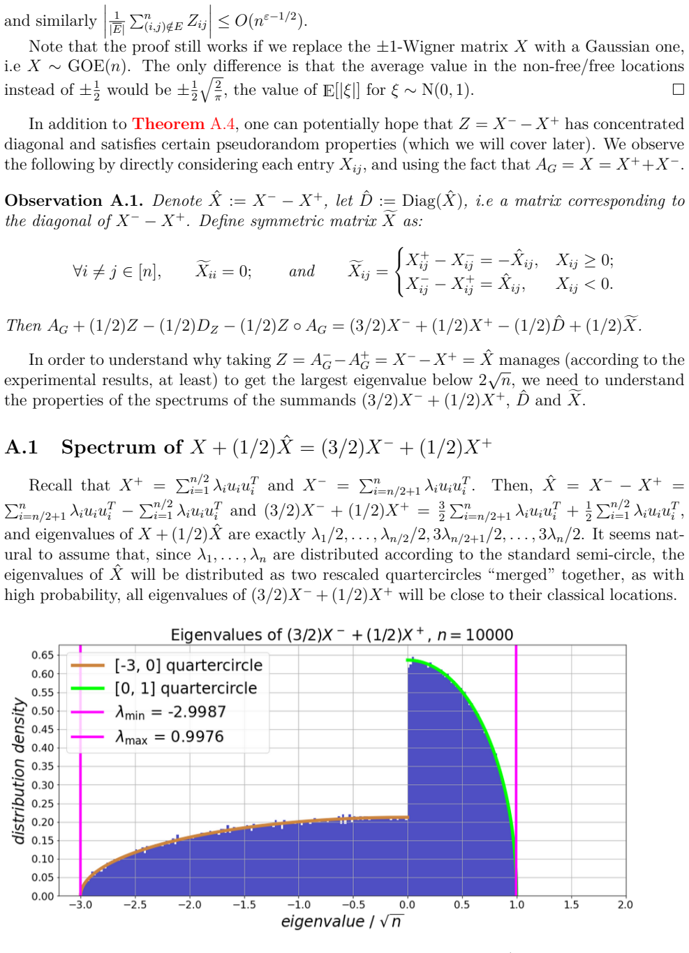
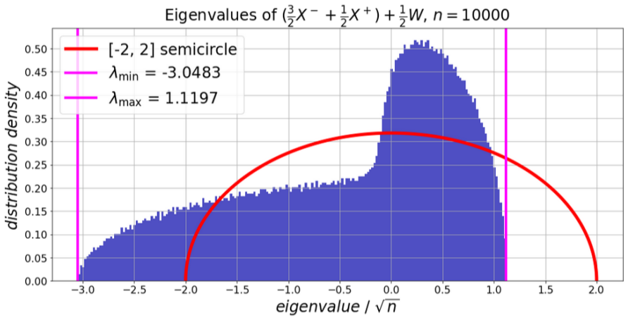
The central object is the spectral sign-flip matrix Z = X− − X+, which has the same eigenvectors as the adjacency matrix X but negated eigenvalues on half of the spectrum. The load-bearing identity is Y = 1/2Z − 1/2D_Z − 1/2Z∘X, rewriting the candidate certificate M = X + Y as (3/2)X− + (1/2)X+ − (1/2)D_hatX + (1/2)tildeX, so that the spectral analysis splits into three pieces: two quarter-circle spectra from X, a concentrated diagonal contribution, and a matrix tildeX that is treated as a generalized Wigner matrix. The free convolution P_{3/2,1/2} ⊞ P_α, with α = $\sqrt$(1 − 64/($9π^{2}$)), shifted up by 4/(3π), is the mechanism that carries the argument from the individual spectra to the predicted top eigenvalue 1.544√n.
What would settle it
Compute λ1(M)/√n for simulated graphs at n = $10^{4}$ and n = $10^{5}$; if for either size the empirical ratio exceeds 1.55 + ε with high probability for some fixed ε > 0, Conjecture 1 is false. Separately, the block-diagonal generalized Wigner matrix described in Section B.3 provides a direct test of Assumption 5: adding a diagonal matrix with two different block signs to that W should change eigenvalues blockwise and fail to match the free-convolution prediction.
Extended reading notes
Core claim
The central claim is Conjecture 1: for the matrix M constructed below, λ1(M) ≤ 1.55√n with high probability, and since M ∈ M_G certifies that ϑbar(G) ≤ λ1(M), this would give E[ϑ(G(n,1/2))] ≤ 1.55√n. The construction takes X to be the ±1 adjacency matrix of G, writes X = X+ + X− where X+ and X− are the positive and negative spectral parts, and sets Z = X− − X+. Then M = X + Y with Y = 1/2Z − 1/2D_Z − 1/2Z∘X, where D_Z is the diagonal of Z and ∘ is entrywise product. The paper analyzes the spectrum of X + (1/2)Z − (1/2)D_Z − (1/2)Z∘X by replacing Z∘X with a sign-randomized matrix W that is a generalized Wigner matrix, computing the free convolution of the two quarter-circle spectrum of X + (1/2)Z with the semicircle spectrum of (1/2)W, and shifting by the diagonal contribution 4/(3π). This predicts λ1(M) ≈ 1.544√n, matching experiments up to n=10000.
Load-bearing premise
The predicted value 1.55√n rests on the unproven assumption that the sign-randomized matrix W is asymptotically free from the deterministic matrix X + (1/2)(X− − X+), so the spectrum of their sum is exactly the free convolution and the largest eigenvalue sticks to its top edge — a property known for Wigner matrices but not for generalized Wigner matrices, which the paper admits can fail.
Editorial extensions
If this is right
- If Conjecture 1 holds, E[ϑ(G(n,1/2))] ≤ 1.55√n, giving the first improvement over Juhász's 2√n bound in over 40 years.
- Every parameter in the new class is polynomial-time computable and certifies an upper bound on the theta function of any graph, not only random graphs.
- Scaling the chosen Z by a factor of 1.3 experimentally lowers the bound to roughly 1.5√n, and a recursive variant of the construction gives roughly 1.45√n experimentally.
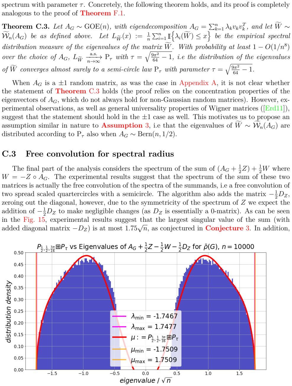
- The same framework applied to spectral radius suggests (Conjecture 3) that ρbar(G) ≤ 1.75√n for G(n,1/2), alongside the paper's rigorous lower bound ρbar(G) ≥ (3π/8−o(1))√n ≈ 1.178√n.
- If the free-convolution prediction is correct, the largest eigenvalue of the constructed matrix sticks to the top endpoint of the predicted support, so the improved bound is a genuine spectrum-level property rather than a lucky outlier.
Reading between the lines
- If the 1.55√n bound is eventually proved, the known gap for ϑ(G(n,1/2)) would shrink from a factor of 2 to a factor of roughly 1.55, and any theta-based statistical test for planted cliques would gain a threshold at 1.55√n instead of 2√n; even below √n, the associated matrices' statistics might give distinguishability where λ1 alone cannot.
- The paper's central open problem, a deterministic version of free convolution for matrices with correlated entries, would also clarify exactly when generalized Wigner matrices are free from deterministic matrices, a regime where the paper itself exhibits a block-diagonal counterexample.
- A direct testable extension is to simulate the constructed M for n beyond 10000 and plot λ1(M)/√n; if the ratio drifts above 1.55 with high probability at any fixed large n, then at least one of the heuristic assumptions fails even if the underlying conjecture about ϑ survives.
- If Assumption 1 (concentrated diagonal) is the only missing piece for Bernoulli matrices, then recent delocalization bounds for eigenvectors of Wigner matrices might be pushed to close the c>1 gap the paper identifies, yielding a rigorous route to the 1.55√n bound.
Editorial analysis
A structured set of objections, weighed in public.
Referee Report
Summary. The paper studies the Lovász theta function on Erdős–Rényi graphs G(n,1/2), for which the long-standing bounds are 1√n and 2√n. It introduces a class of polynomial-time computable graph parameters that upper-bound the theta function: given the ±1 adjacency matrix X of G, a matrix Z is chosen with the same eigenbasis as X, and the candidate matrix M = X + Y is formed by replacing only the free entries of X with the corresponding entries of Z. The paper rigorously proves Proposition 1.1, showing that independent choices of the free entries cannot beat 2√n, and Theorem 1.1, a new lower bound (3π/8−o(1))√n on the spectral-radius parameter ρ̄(G). The main positive claim is Conjecture 1: for the specific choice Z = X− − X+, λ1(M) ≤ 1.55√n with high probability, which would imply E[ϑ(G(n,1/2))] ≤ 1.55√n. The argument for this value is a five-step heuristic analysis under Assumptions 1–5, combined with free-probability computations of the spectrum of the sum. A similar conditional treatment (Conjecture 2/3) is given for the spectral radius, with predicted value 1.75√n. The paper explicitly states that it falls short of a rigorous proof.
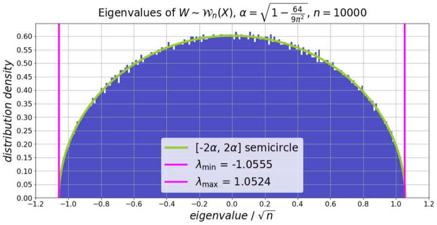
Significance. If Conjecture 1 were established, it would improve Juhász's 40-year-old upper bound 2√n and would constitute a first qualitative improvement of the trivial matrix-based bound. The paper also contributes several rigorous results: Proposition 1.1 rules out a natural class of independent free-entry constructions; Theorem 1.1 gives a new lower bound on ρ̄(G); and the appendices prove concentration results for diagonal and generalized-Wigner objects in the Gaussian case (Theorems E.1, F.1, and related statements). A notable strength is that the predicted constants are not fitted to the theta values: α = √(1−64/(9π²)) and the 4/(3π) shift derive analytically from the spectrum of the chosen Z, and the free convolution is computed from those derived spectra. The central limitation is that the 1.55√n claim is conditional on unproven structural assumptions, especially Assumption 5 on asymptotic freeness, which the paper itself notes is not known for generalized Wigner matrices and for which it provides a related counterexample.
major comments (4)
- [B.3, Assumption 5] The derivation of the predicted largest eigenvalue 1.544√n, and hence Conjecture 1, rests on Assumption 5: that A = (3/2)X− + (1/2)X+ and (1/2)W are asymptotically free, that their sum converges to the free convolution P_{3/2,1/2} ⊞ P_α, and that λ1 sticks to the support of that convolution. This is load-bearing: without it, the free-convolution computation has no proven application to the actual matrix sum, and the number 1.55√n is unsupported by the analytical framework. The paper itself states in Section B.3 that generalized Wigner matrices are not known to be free even with deterministic diagonal matrices, and gives a block-diagonal example where freeness fails. In the present construction W is not independent of A: the variances of W are determined by the eigenvectors of X, which also define A. That correlation is precisely the type of structure that can destroy free independence. As the paper is honest about, this gap leaves Conjecture 1 as an empirical conjecture rather than a consequence of the stated free-probability analysis.
- [1.6, step 4; A.4, Assumptions 2 and 4] The analysis replaces the actual matrix ~X = Z∘A_G by the sign-randomized generalized Wigner matrix W ∼ W_n(X), first for the individual spectrum (Assumption 2) and then for the spectrum of the sum with A (Assumption 4). Even if the empirical spectral distributions of ~X and W converge to the same limit, this does not imply that their eigenbases are similarly aligned with the eigenbasis of A; the spectral distribution of A + ~X can differ from that of A + W. Assumption 4 is exactly the additional input needed, and the paper says that proving it 'seems beyond reach of current techniques.' Since the subsequent free-convolution step is applied to the sum with W, rather than to ~X, the actual matrix M used in Conjecture 1 is not covered without Assumption 4. This is a second independent load-bearing gap.
- [1.7, step 2; G, Theorem G.1] The derivation of the 4/(3π)√n shift, used to obtain λ1(A + (1/2)Z − (1/2)D_Z) ≈ (1 + 4/(3π))√n, relies on the diagonal of X− − X+ being simultaneously concentrated around a common value ν (Assumption 1). For the Gaussian case this is proved in Theorem E.1, but for the ±1 Wigner case Theorem G.1 only gives per-entry concentration of each diagonal entry with failure probability of order 1/(t²√n), which is not enough to union bound over all n entries. The paper explicitly notes that it 'comes very close' but cannot obtain the simultaneous concentration needed. Without Assumption 1, the diagonal matrix is not (ν+o(1))I with high probability, and the additive spectral shift is not justified.
- [C, Conjectures 2 and 3] The spectral-radius upper bound 1.75√n in Conjecture 2/3 is subject to the same type of unproven assumptions as Conjecture 1: the spectral analysis of Z∘A_G replaces it by a generalized Wigner matrix, assumes the spectra of the sums are similar, and then assumes asymptotic freeness and edge sticking. These are stated in Appendix C as assumptions of the same nature as Assumptions 2, 4, and 5. Since this is one of the paper's two main conjectured contributions, the conditional nature of the bound should be made explicit in the theorem statements, not only in the introductory discussion.
minor comments (5)
- [Abstract and Title] The title and abstract say 'upper bounds on the theta function,' but the 1.55√n bound is a conjecture conditional on unproven assumptions. Suggest changing the wording to 'conditional upper bounds' or 'heuristic evidence for improved upper bounds' to match the content.
- [1.8 vs. C] The conjecture about the spectral radius is labelled Conjecture 2 in Section 1.8 but is called Conjecture 3 in Appendix C. The numbering should be made consistent.
- [1.6, Eq. (1)] The notation D_Z is used before it is explicitly defined as the diagonal matrix whose diagonal is that of Z. Please define it at first use.
- [Throughout] The notation M ∈ M_G in Definition 1.1 becomes M ∈ M(G) in Section C. These should be unified.
- [Figures] Several figures (e.g., Figures 1, 2, 9–12) are central to the empirical evidence, but no details are given about the number of samples, error bars, or whether the experiments are reproducible from provided code. Adding a short experimental methodology paragraph would strengthen the paper.
Circularity Check
No circularity: the 1.55√n bound is an explicitly unproven heuristic conjecture whose constants are derived analytically from the chosen matrix Z, not fitted to theta-function values.
full rationale
The paper's central claim, Conjecture 1, is that λ1(M) ≤ 1.55√n with high probability for a specific M ∈ M_G, and the analysis supporting it is heuristic rather than circular. The constants entering the prediction are computed analytically: the diagonal shift 4/(3π)√n comes from the trace of Z (Lemma A.2), the semicircle width α = sqrt(1−64/(9π²)) comes from the Frobenius norm of Z minus its diagonal (Corollary F.1), and the final 1.544√n comes from numerically evaluating the free convolution P_{3/2,1/2} ⊞ P_α, a distribution determined by the spectrum of (3/2)X⁻+(1/2)X⁺ and the variance profile of W. None of these constants is fit to the experimental theta values; the agreement with experiments is presented as evidence for the unproven Assumptions 2–5, not as input to the calculation. The main weakness is Assumption 5, which asserts asymptotic freeness of a deterministic matrix and a generalized Wigner matrix, and the paper explicitly states this is not known and gives a counterexample to generic freeness. However, an unproven assumption is not circular: the conjecture would follow if the assumption were true, and the paper does not use Conjecture 1 itself as an input. Self-citations in the paper are to prior planted-clique and theta-related work and are not load-bearing for the derivation. Thus there is no step where a prediction reduces by construction to a fitted parameter or to a self-citation chain.
Assumptions & free parameters
free parameters (2)
- τ (scaling of Y in Section 1.9) =
≈1.3
- Z' scaling factor =
1.3
assumptions (8)
- standard math Wigner semicircle law, eigenvalue rigidity, and eigenvector delocalization for ±1 Wigner matrices.
- standard math Free convolution describes spectra of sums of asymptotically free random/deterministic matrices, and λ1 sticks to the support under the conditions of Theorem B.5.
- standard math Gaussian eigenvectors are independent of eigenvalues and uniformly distributed (Theorem E.2).
- ad hoc to paper Diagonal entries of X_- - X_+ are simultaneously concentrated around one value ν, with failure probability O(n^{-K}).
- ad hoc to paper Empirical spectral distribution of ~X = Z∘AG equals that of the sign-randomized generalized Wigner W.
- ad hoc to paper The sign-randomized matrix W has a semicircular limiting spectrum with some α for ±1 Wigner X.
- ad hoc to paper The sum (3/2)X_-+(1/2)X_+ + (1/2)~X has the same limiting spectrum as the sum with (1/2)W.
- ad hoc to paper X+(1/2)Xhat and (1/2)W are asymptotically free; the sum's spectrum is the free convolution P_{3/2,1/2}⊞Pα; λ1 sticks to the support.
Cite this review
Pith. "Pith review of Upper bounds on the theta function of random graphs." pith.science (2026). https://pith.science/paper/DHRTS66O
@misc{pith2026250602952,
  author       = {Pith},
  title        = {Pith review of: Upper bounds on the theta function of random graphs},
  year         = {2026},
  howpublished = {\url{https://pith.science/paper/DHRTS66O}},
  note         = {Machine review of arXiv:2506.02952}
}
abstract
The theta function of Lovasz is a graph parameter that can be computed up to arbitrary precision in polynomial time. It plays a key role in algorithms that approximate graph parameters such as maximum independent set, maximum clique and chromatic number, or even compute them exactly in some models of random and semi-random graphs. For Erdos-Renyi random $G_{n,1/2}$ graphs, the expected value of the theta function is known to be at most $2\sqrt{n}$ and at least $\sqrt{n}$. These bounds have not been improved in over 40 years. In this work, we introduce a new class of polynomial time computable graph parameters, where every parameter in this class is an upper bound on the theta function. We also present heuristic arguments for determining the expected values of parameters from this class in random graphs. The values suggested by these heuristic arguments are in agreement with results that we obtain experimentally, by sampling graphs at random and computing the value of the respective parameter. Based on parameters from this new class, we feel safe in conjecturing that for $G_{n,1/2}$, the expected value of the theta function is below $1.55 \sqrt{n}$. Our paper falls short of rigorously proving such an upper bound, because our analysis makes use of unproven assumptions.
Figures


Figures from the paper (12 more)




Reference graph
Works this paper leans on
-
[3]
1 n ∑n i=1 ⏐⏐⏐1 n ∑n j=1σ2 ij− 1 ⏐⏐⏐ n→∞ −−−→0. Then, LW a.s. −−−→n→∞ P, where P is the standard semi-circle law. Supporting Theorem A.10, numerical experiments with X∼ Bern±1(n, 1/2) show (Fig. 6) that the spectrum ofW∼W n(X) is distributed like a scaled standard semi-circle, with a scaling parameter essentially the same as the one we had for the matrix ...
-
[4]
= φ(a1a′ 1)φ(a2) andφ(a1a2a′ 1a′
-
[5]
=φ(a1a′ 1)φ(a2)φ(a′ 2)+φ(a1)φ(a′ 1)φ(a2a′ 2)−φ(a1)φ(a′ 1)φ(a2)φ(a′ 2). In order to derive these equalities, we rely on the fact from Definition B.1 that the mixed mo- ments of centered random variances must be equal to 0. For example, the first equality is obtained as follows: φ [(a1−φ(a1)1)(a2−φ(a2)1)(a′ 1−φ(a′ 1)] = 0 =⇒ φ [a1a2a′ 1−φ(a1)a2a′ 1−a1φ(a2)a...
-
[6]
+a1φ(a2)φ(a′ 1)−φ(a1)φ(a2)φ(a′ 1)1] = 0 =⇒ φ(a1a2a′ 1)−φ(a1)φ(a2a′ 1)−φ(a2)φ(a1a′
-
[7]
+φ(a1)φ(a2)φ(a′ 1)− φ(a1a2)φ(a′
-
[8]
+φ(a1)φ(a2)φ(a′ 1)−φ(a1)φ(a2)φ(a′
-
[9]
33 Now, using the fact that a2 is free from a1 anda′ 1, we haveφ(a1a2) =φ(a1)φ(a2) and φ(a2a′
= 0. 33 Now, using the fact that a2 is free from a1 anda′ 1, we haveφ(a1a2) =φ(a1)φ(a2) and φ(a2a′
-
[10]
= φ(a2)φ(a′ 1). Then, after cancellations, the only terms left are φ(a1a2a′ 1)−φ(a1a′ 1)φ(a2) = 0. Even though free independence was developed as an analogue to classical, commutative independence, it is not a generalization. Classical commuting random variables a1,a 2 are free only in the trivial case (when either a1 or a2 is a constant). Indeed, in comm...
Show all 20 references
-
[11]
µa has compact support [sa,ta], µb has compact support [sb,tb]
-
[12]
µa has sqrt-behaviour, µb is a Jacobi measure
-
[13]
Letg(z) := G−1 µa⊞µb(z) = G−1 µa (z) +G−1 µb (z)− 1 z
Cauchy transforms Gµa,Gµn are invertable. Letg(z) := G−1 µa⊞µb(z) = G−1 µa (z) +G−1 µb (z)− 1 z . Then the support of µa ⊞µb is contained in the interval [s,t ] = [gs,gt] wheregs,gt are unique zeroes of the derivative g′(z) in the intervals ( max{Gµa(sa),Gµb(sb)}, 0 ) and ( 0,...
-
[14]
matrices X + (1/2) ˆX and (1/2)W are asymptotically free
-
[15]
the empirical spectral distribution measure of X +(1/2) ˆX +(1/2)W converges to P 3 2, 1 2 ⊞Pα
-
[16]
This does indeed seem to be true, according to experimental results, as one can see in Fig
for every ε> 0, for all large n, spec(X + (1/2) ˆX + (1/2)W )⊂ supp(P 3 2, 1 2 ⊞ Pα) + (−ε,ε ) with probability tending to 1 as n→∞ ; Following the discussion regarding the eigenvalues of the diagonal matrixˆD, (Assumption 1 and Theorem A.9), we expect that zeroing-out the dia...
-
[17]
≥λn, then ∑ k:λk≥0 λk = 4 3πn3/2±O(n1/2 polylogn) and ∑ k:λk≤0 λk =− 4 3πn3/2±O(n1/2 polylogn)
if AG =∑n k=1λkukuT k is an eigendecomposition of AG, and λ1≥... ≥λn, then ∑ k:λk≥0 λk = 4 3πn3/2±O(n1/2 polylogn) and ∑ k:λk≤0 λk =− 4 3πn3/2±O(n1/2 polylogn). Proposition D.1. With probability at least 1−O(n−1 polylogn), graphG∼G(n, 1/2) is typical. Proof. For the first cond...
-
[18]
The collection [u1,...,u n] is independent of the eigenvalues λ1,...,λ n, and each of the eigenvectorsu1,...,u n is distributed uniformly on Sn−1 + ={x∈ Rn :∥x∥ = 1,x 1 > 0}
-
[19]
U = [u1,...,u n] is distributed according to Haar measure on O(n) (orthogonal matrices of size n), with each ui multiplied by a±1-scalar so that all columns of U belong to Sn−1 + . Applying Theorem E.2 to Y , it is easy to see that by independence of λi-s and ui-s E [ Y + kk ]...
-
[20]
for any constant η >0, limn→∞ 1 n2 ∑n i,j=1 E [ W 2 ij I{|Wij|>η√n} ] = 0
-
[21]
there exists global constant C such that for every i∈ [n], 1 n ∑n j=1σ2 ij≤C
-
[22]
Theorem F.2 gives sufficient conditions for the pointwise convergence of E[LW ] to Pα for some α> 0 (after rescaling)
1 n ∑n i=1 ⏐⏐⏐1 n ∑n j=1σ2 ij− 1 ⏐⏐⏐ n→∞ −−−→0; then supx∈R|E[LW (x)]− P1(x)| n→∞ −−−→0, where P1 is the standard semicircle law on [−2, 2]. Theorem F.2 gives sufficient conditions for the pointwise convergence of E[LW ] to Pα for some α> 0 (after rescaling). To obtain almost ...
Reviewed August 7, 2026 · model on record in the stance chip above.
Discussion (0). Sign in to comment.