REVIEW 4 major objections 5 minor 23 references
A randomized progressive iterative regularization method for data fitting problems
T0 review · 4 major / 5 minor · reviewed 2026-08-07 · deepseek-v4-flash
Pith's one-line read Randomized progressive iterative fitting converges in expectation to the regularized least-squares solution, and the paper derives a noise-based formula for the optimal smoothing parameter.
desk verdict A correct but routine convergence theory for regularized randomized PIA, with a self-consistent lambda-selection heuristic that is the real practical claim and the part that lacks proof. read the letter →
The pith
A machine-rendered reading of the paper's core claim, the machinery that carries it, and where it could break.
The reading
What carries the argument
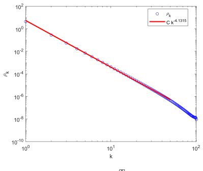
The engine of the argument is the augmented collocation matrix $\hat A = [A; \sqrt{\lambda}\Gamma]$ (and its two-factor tensor form $\hat A P \hat B^T$ for surfaces), which converts Tikhonov regularization into an ordinary least-squares problem. The convergence proof rests on the conditional-expectation identity $\mathbb{E}[z^{(k+1)}] = (I - \hat A \hat A^T/\|\hat A\|_F^2) z^{(k)}$, where $z^{(k)} = \hat A(p^{(k)} - p^*)$; this identity turns the random block update into a deterministic contraction in expectation. For parameter selection, the load-bearing object is the eigenvalue decay assumption $\rho_k \le C k^{-\alpha}$ of $Q^T Q$, which converts the variance term into $\lambda^{-1/\alpha}$ and makes the bias-variance balance yield $\lambda^{1+1/\alpha} = O(\sigma^2 n^{-1})\|\Gamma \bar p\|_n^{-2}$. The self-consistent algorithm in Section 6 iterates that formula by substituting the observed residual ratio for the unknown true ratio.
What would settle it
A direct test is to run the self-consistent fixed-point algorithm on a synthetic B-spline problem with known ground truth $\bar p$, known noise variance $\sigma^2$, and a deliberately misspecified spectral decay rate $\alpha$ (for instance, off by a factor of two); if the converged $\lambda$ moves away from the empirically optimal value that minimizes prediction error, the claim that the algorithm selects the optimal regularization parameter without prior information is falsified.
Extended reading notes
Core claim
On the paper's own terms, the contribution is twofold. First, the regularized RPIA update is shown to be a randomized block-coordinate iteration on the augmented least-squares problem $\min_p \|\hat A p - \hat q\|_F^2$ with $\hat A = [A^T, \sqrt{\lambda}\Gamma^T]^T$. Writing $p^*$ for the Tikhonov solution, the proof tracks $z^{(k)} = \hat A(p^{(k)} - p^*)$ and shows that conditional on the history, the expected next iterate is $(I - \hat A \hat A^T / \|\hat A\|_F^2) z^{(k)}$, a contraction whose spectral radius is below one when $\hat A$ has full column rank; hence $\mathbb{E}[p^{(k)}] \to p^*$ for curves, and a tensor-product analogue gives the same for surfaces. Second, for noisy data $q_e = A\bar p + \epsilon + e$ with i.i.d. noise of variance $\sigma^2$ and eigenvalue decay $\rho_k \le C k^{-\alpha}$, the paper proves the mean squared prediction error is bounded by $C\lambda\|\Gamma \bar p\|^2 + C(\sigma^2 + \sum_i \epsilon_i^2)/\lambda^{1/\alpha}$, and balancing these terms yields the optimal-parameter formula. The same formula then motivates a self-consistent fixed-point iteration that estimates $\lambda$ from the current fit rather than from known noise levels.
Load-bearing premise
The load-bearing premise is that, inside the self-consistent parameter algorithm, the quantity $\|A p^{(k)} - q_{\text{noise}}\|_m^2 / (\|\Gamma p^{(k)}\|_n^2 \, n^{-1})$ can stand in for the true but unknown $\sigma^2 / \|\Gamma \bar p\|^2$, that the fixed point of this substitution is the minimizer of the true prediction error, and that the user knows the spectral decay rate $\alpha$; none of this is proved.
Editorial extensions
If this is right
- For curve and surface fitting with noisy data, the randomized block iteration gives the Tikhonov solution in expectation, so standard regularization guarantees carry over while each step keeps the low per-iteration cost of RPIA.
- The parameter rule $\lambda^{1+1/\alpha} = O(\sigma^2 n^{-1})\|\Gamma \bar p\|_n^{-2}$ predicts that optimal smoothing grows with noise level and shrinks with the number of data points, a trend the experiments confirm when the noise amplitude rises from 40 to 100.
- In the surface case, regularization factorizes into separate $u$- and $v$-direction penalties and the method drops the $\lambda^2$ cross term; for the small $\lambda$ values reported, that discarded term is numerically harmless.
- Because convergence is in expectation, averaging several independent runs reduces random-block variance and is part of the practical recipe the experiments use.
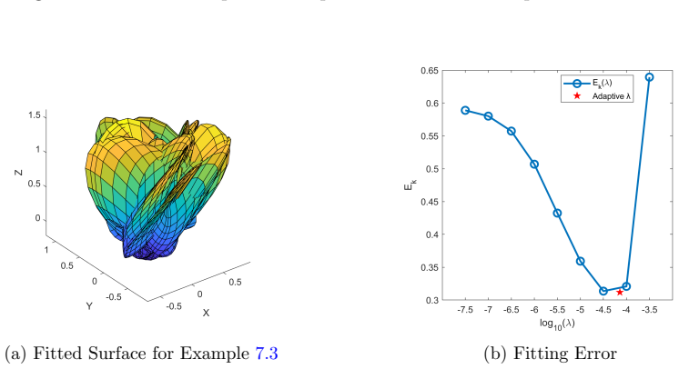
- The self-consistent parameter iteration reaches fitting errors at or below the non-adaptive parameter choice in the reported examples, which suggests the residual-based estimate works as a usable discrepancy principle.
Reading between the lines
- The paper does not analyze the variance of the randomized estimator around its expectation; an unstated practical consequence is that the number of independent runs needed for a reliable fit should grow with the condition number of $\hat A$.
- The fixed-point update can be read as a randomized discrepancy principle; a natural extension is to replace the in-sample residual with a cross-validated residual when deterministic model error dominates measurement noise, since the bound contains an extra $\sum_i \epsilon_i^2$ term the algorithm currently ignores.
- The optimal-$\lambda$ formula depends on the spectral decay exponent $\alpha$, which the paper measures from the eigenvalue plot of $Q^T Q$; estimating $\alpha$ online from the same iterates would be needed to make the 'without prior information' claim literally true.
- The parameter loop assumes the augmented least-squares problem is solved at each fixed-point step, while the fitting itself is iterative; how early stopping of the inner iteration changes the fixed point of $\lambda$ is left unexamined.
Editorial analysis
A structured set of objections, weighed in public.
Referee Report
Summary. The paper proposes a randomized progressive iterative regularization method (regularized RPIA) for noisy curve and surface fitting. The method applies block-coordinate updates to the Tikhonov-augmented least-squares problem, and the authors prove that the resulting iteration converges in expectation to the augmented least-squares solution (Theorems 4.1 and 4.2). They then derive a stochastic bias-variance bound for the regularized estimate (Theorem 5.1) and use it to propose an order-optimal regularization parameter formula, leading to a self-consistent fixed-point algorithm (Section 6) intended to select λ without prior noise level information. Three numerical experiments (two curves, one surface) are reported to illustrate the theoretical analysis and the performance of the adaptive parameter selection.
Significance. If the parameter-selection algorithm were rigorously justified, the paper would provide a practical randomized method for large-scale noisy data fitting with an automatic regularization parameter choice. The convergence-in-expectation proof is a clean extension of the RPIA analysis and is the sound core of the paper. The bias-variance bound in Theorem 5.1 is a standard but useful result, and the optimal λ formula is derived from the bound rather than fitted to numerical error curves, which is a strength. The main weakness is that the self-consistent algorithm, advertised as a third contribution, is heuristic: no convergence or optimality statement is proved, and the 'without prior information' claim is overstated because the spectral decay rate α is required as an input.
major comments (4)
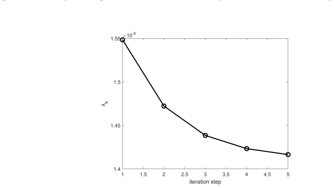
- [Section 6, Tables 6.1/6.2] The self-consistent fixed-point algorithm is presented as the paper's third contribution ('self-consistent algorithms without prior information'), but no theorem establishes that the sequence λ_k converges, that a fixed point exists or is unique, or that the fixed point is close to the minimizer of the true prediction error. The update rule replaces the unknown noise variance σ^2 by the empirical residual norm ||Ap^{(k)}−q_noise||_m^2, which contains a regularization-bias term, and replaces ||Γpbar||_n by the systematically smaller ||Γp^{(k)}||_n; these substitutions are not justified. The algorithm also requires the spectral decay rate α as an input, contradicting the 'without prior information' claim. The numerical evidence in Section 7.3 consists of three examples with means only, no error bars, and does not settle the convergence or optimality question.
- [Section 5, Theorem 5.1 proof, Eqs. (5.4)-(5.5)] The proof contains a normalization inconsistency with Assumption 1. Assumption 1 states that the eigenvectors φ_k form an orthonormal basis, but the proof sets (φ_k, φ_k) = 1/ρ_k. Under true orthonormality one would have (u,u) = Σ (u,φ_k)^2 and (Qu,Qu) = Σ ρ_k (u,φ_k)^2, not the formulas in (5.4)-(5.5). The subsequent derivation requires a rescaled basis satisfying (Qφ_k,Qφ_k)=1 and (φ_k,φ_k)=1/ρ_k, which is not the basis described in the assumption. The assumption and proof must be reconciled, for example by explicitly stating that the basis is orthogonal with those norms.
- [Abstract and Theorem 4.1] The abstract and introduction claim that the method 'converges to the least-squares solution'; Theorem 4.1 actually proves convergence in expectation to the least-squares solution of the augmented system (Âp = q̂), i.e., to the Tikhonov-regularized solution for a fixed λ. This is not the unregularized least-squares solution of the original problem. In addition, the phrase 'under a certain level of noise' is not connected to any hypothesis in Theorem 4.1, which holds for any λ>0. The wording should be corrected to avoid overclaiming.
- [Remark 5.1 and Section 6] The optimal parameter formula λ^{1+1/α}=O(σ^2 n^{-1})||Γpbar||_n^{-2} is obtained by balancing the two terms of an upper bound, so the proportionality constant is not determined. The self-consistent algorithm in Tables 6.1 and 6.2 fixes the constant to 1 without justification. Furthermore, the claim that the estimated λ is 'very close' to the empirical optimum is supported only by visual inspection of Figures 2(d), 4(d), 5(d), and 7(d); for a quantitative parameter-selection claim, the paper should provide repeated-trial statistics (e.g., standard errors) or a theoretical error bound on the selected λ.
minor comments (5)
- [Throughout] There are several typos and grammatical slips, e.g., 'arrvies' in the proof of Theorem 5.1 and 'It achieves that' in the proof of Theorem 4.2; these should be corrected in a revision.
- [Theorem 4.2 proof] In the denominator after the conditional expectation for surfaces, the term '||B̂V_{sk}||_F^2' and later '||B̂^T||_F^2' should be consistently written as '||B̂||_F^2'.
- [Section 3.2 and Table 6.2] The surface regularization problem includes a λ^2 term, but the parameter-estimation update in Table 6.2 omits it; the text in Section 7.2 states that the high-order term is discarded, but no justification is given beyond the observation that λ is small. A comment in Section 6 would clarify this approximation.
- [Section 7.3] The results of the self-consistent algorithm are reported as arithmetic means of 10 (curves) or 3 (surfaces) runs, but no standard deviations or confidence intervals are given, making it difficult to judge the reliability of the reported improvements.
- [Section 7, fitting error definition] In the fitting error definitions Ek(λ) = ||Ap∗−A p̄||_F^2 / ||A p̄||_F^2 (and the surface analogue), the notation p∗ refers to the regularized solution; this should be stated explicitly to avoid confusion with the unregularized least-squares solution.
Circularity Check
No circularity: the convergence proof and the optimal-regularization-parameter bound are self-contained; the unproven fixed-point lambda iteration is a missing-proof concern, not a circular reduction.
full rationale
The paper's main derivation chain is self-contained. Theorem 4.1 proves convergence in expectation of the regularized RPIA by analyzing the recurrence E[z^(k+1)] = (I - Ahat Ahat^T / ||Ahat||_F^2) E[z^(k)] and using only the positive definiteness of Ahat^T Ahat; no fitted quantity or prior result is needed for the key step, and the surface case in Theorem 4.2 is the same argument with Kronecker products. The optimal-regularization-parameter formula in Remark 5.1 is obtained by balancing the two terms of the derived mean-squared-error bound, not by fitting the numerical error curves: the bound has the form C n lambda/m ||Gamma pbar||_n^2 + C(sigma^2 + sum epsilon_i^2)/(m lambda^(1/alpha)), and equating the leading terms gives lambda^(1+1/alpha) = O(sigma^2 n^{-1}) ||Gamma pbar||_n^{-2}. This is a bias-variance tradeoff derived from the stochastic estimate, so the claimed optimal parameter is not equivalent to the input data by construction. Section 6's self-consistent fixed-point iteration is a heuristic replacement of the unknown sigma^2 and ||Gamma pbar||_n by the current residual and ||Gamma p^(k)||_n; no theorem proves that its fixed point coincides with the minimizer of the true expected error, but that absence is a correctness or rigor gap, not circularity, because the update is not asserted to be equivalent to the derived optimum. The paper does not contain load-bearing self-citation: the cited RPIA work [18] is the base algorithm, while the convergence and parameter estimates are proved in the present paper. The numerical validation compares the formula with true error curves on synthetic examples with known ground truth; even though alpha is estimated from the spectrum of Q, the reported lambda values are not, by the paper's own account, fitted to the error minima. Overall, the central claims are independent of their inputs, so the circularity score is 0.
Assumptions & free parameters
free parameters (3)
- spectral decay rate alpha =
4.1315 (Ex 7.1), 4.1317 (Ex 7.2), 2.0929 (Ex 7.3)
- regularization matrix scale C =
C = 1600 in curve examples, C = 91 in surface example
- initial regularization parameter lambda_1 =
lambda_1^(1+1/alpha) = n^{-1}
assumptions (5)
- domain assumption Assumption 1: eigenvalues rho_k of (Q phi, Q u) = rho(phi, u) decay as rho_k <= C k^{-alpha}
- domain assumption Noise model: q_e = q + e with e_i i.i.d., E[e_i]=0, E[e_i^2]=sigma^2
- ad hoc to paper Small model error: q = A pbar + epsilon with epsilon very small relative to e
- standard math Full-column rank of A and of Ahat = [A; sqrt(lambda)Gamma]
- standard math Gamma is invertible and B = Gamma^{-1} exists
Cite this review
Pith. "Pith review of A randomized progressive iterative regularization method for data fitting problems." pith.science (2026). https://pith.science/paper/VJPJHJ4J
@misc{pith2026250603526,
  author       = {Pith},
  title        = {Pith review of: A randomized progressive iterative regularization method for data fitting problems},
  year         = {2026},
  howpublished = {\url{https://pith.science/paper/VJPJHJ4J}},
  note         = {Machine review of arXiv:2506.03526}
}
read the original abstract
In this work, we investigate data fitting problems with random noises. A randomized progressive iterative regularization method is proposed. It works well for large-scale matrix computations and converges in expectation to the least-squares solution. Furthermore, we present an optimal estimation for the regularization parameter, which inspires the construction of self-consistent algorithms without prior information. The numerical results confirm the theoretical analysis and show the performance in curve and surface fittings.
Figures


Figures from the paper (12 more)



Reference graph
Works this paper leans on
-
[1]
A variational non-linear constrained model for the inversion of fdem data
Alessandro Buccini and Patricia Diaz de Alba. A variational non-linear constrained model for the inversion of fdem data. Inverse Problems, 38, 2021
work page 2021
-
[2]
Distributed tikhonov regularization for ill- posed inverse problems from a bayesian perspective
Daniela Calvetti and Erkki Somersalo. Distributed tikhonov regularization for ill- posed inverse problems from a bayesian perspective. Computational Optimization and Applications, 2025. 26
work page 2025
-
[3]
J.M. Carnicer, J. Delgado, and J.M. Pe˜ na. Richardson method and totally non- negative linear systems. Linear Algebra and its Applications , 433(11):2010–2017, 2010
work page 2010
-
[4]
de Boor C. How does agee’s smoothing method work? In Proceedings of the 1979 Army Numerical Analysis and Computers Conference , ARO Report 79-3, pages 299–302. Army Research Office, 1979
work page 1979
-
[5]
Progressive and iterative approximation for least squares b-spline curve and surface fitting
Chongyang Deng and Hongwei Lin. Progressive and iterative approximation for least squares b-spline curve and surface fitting. Computer-Aided Design, 47:32–44, 2014
work page 2014
-
[6]
A. Ebrahimi and G.B. Loghmani. A composite iterative procedure with fast con- vergence rate for the progressive-iteration approximation of curves. Journal of Computational and Applied Mathematics , 359:1–15, 2019
work page 2019
-
[7]
On a progressive and iterative approximation method with memory for least square fitting
Zheng-Da Huang and Hui-Di Wang. On a progressive and iterative approximation method with memory for least square fitting. Computer Aided Geometric Design , 82:101931, 2020
work page 2020
-
[8]
Totally positive bases and pro- gressive iteration approximation
Hong-Wei Lin, Hu-Jun Bao, and Guo-Jin Wang. Totally positive bases and pro- gressive iteration approximation. Computers & Mathematics with Applications , 50(3):575–586, 2005
work page 2005
Show all 23 references
-
[9]
Local progressive-iterative approximation format for blending curves and patches
Hongwei Lin. Local progressive-iterative approximation format for blending curves and patches. Computer Aided Geometric Design , 27(4):322–339, 2010
2010
-
[10]
Survey on geometric iter- ative methods and their applications
Hongwei Lin, Takashi Maekawa, and Chongyang Deng. Survey on geometric iter- ative methods and their applications. Computer-Aided Design, 95:40–51, 2018
2018
-
[11]
An extended iterative format for the progressive- iteration approximation
Hongwei Lin and Zhiyu Zhang. An extended iterative format for the progressive- iteration approximation. Computers & Graphics , 35(5):967–975, 2011
2011
-
[12]
Preconditioned progressive iterative approximation for triangular b´ ezier patches and its application
Chengzhi Liu, Xuli Han, and Juncheng Li. Preconditioned progressive iterative approximation for triangular b´ ezier patches and its application. Journal of Com- putational and Applied Mathematics , 366:112389, 2020
2020
-
[13]
Weighted progressive iteration approximation and convergence anal- ysis
Lizheng Lu. Weighted progressive iteration approximation and convergence anal- ysis. Computer Aided Geometric Design , 27(2):129–137, 2010
2010
-
[14]
A regularization approach for sur- face reconstruction from point clouds
Hebert Montegranario and Jairo Espinosa. A regularization approach for sur- face reconstruction from point clouds. Applied Mathematics and Computation , 188(1):583–595, 2007
2007
-
[15]
Uniform b-spline curve interpolation with prescribed tan- gent and curvature vectors
Shoichi Okaniwa, Ahmad Nasri, Hongwei Lin, Abdulwahed Abbas, Yuki Kineri, and Takashi Maekawa. Uniform b-spline curve interpolation with prescribed tan- gent and curvature vectors. IEEE Transactions on Visualization and Computer Graphics, 18(9):1474–1487, 2012
2012
-
[16]
D. Qi, Z. Tian, Y. Zhang, and J. Feng. The method of numeric polish in curve fitting. ACTA MATHEMATICA SINICA, 18(3):173–184, 1975
1975
-
[17]
Lspia, (stochastic) gradient descent, and parameter correction
Dany Rios and Bert J¨ uttler. Lspia, (stochastic) gradient descent, and parameter correction. Journal of Computational and Applied Mathematics , 406:113921, 2022
2022
-
[18]
Randomized progressive iterative approximation for b-spline curve and surface fittings
Nian-Ci Wu and Cheng-Zhi Liu. Randomized progressive iterative approximation for b-spline curve and surface fittings. Applied Mathematics and Computation , 473:128669, 2024
2024
-
[19]
On the triple-parameter least squares progressive iterative approximation and its convergence analysis
Nian-Ci Wu, Chengzhi Liu, and Juncheng Li. On the triple-parameter least squares progressive iterative approximation and its convergence analysis. Computer Aided Geometric Design, 119:102439, 2025
2025
-
[20]
Curve fitting of the user barrage emotional change based on the hybrid kernel pso lssvm model
Fulian Yin, Xiaoli Feng, Fangyuan Ju, and Yanyan Wang. Curve fitting of the user barrage emotional change based on the hybrid kernel pso lssvm model. Proceedings of the 2020 3rd International Conference on Algorithms, Computing and Artificial Intelligence, 2020. 27
2020
-
[21]
Impulse noise image restoration using nonconvex variational model and dif- ference of convex functions algorithm
Benxin Zhang, Guopu Zhu, Zhibin Zhu, Hongli Zhang, Yicong Zhou, and Sam Kwong. Impulse noise image restoration using nonconvex variational model and dif- ference of convex functions algorithm. IEEE Transactions on Cybernetics, 54:2257– 2270, 2022
2022
-
[22]
Generalized b-splines’ geomet- ric iterative fitting method with mutually different weights
Li Zhang, Jieqing Tan, Xianyu Ge, and Guo Zheng. Generalized b-splines’ geomet- ric iterative fitting method with mutually different weights. Journal of Computa- tional and Applied Mathematics , 329:331–343, 2018. The International Conference on Information and Computational S...
2018
-
[23]
Parametric surface reconstruction from 3d point data using partial differential equation and bilinearly blended coons patch
Zaiping Zhu, Shuangbu Wang, Lihua You, and Jianjun Zhang. Parametric surface reconstruction from 3d point data using partial differential equation and bilinearly blended coons patch. Journal of Computational Physics , 519:113436, 2024. 28
2024
Reviewed August 7, 2026 · model on record in the stance chip above.
Discussion (0). Sign in to comment.