REVIEW 4 major objections 4 minor 44 references
Analyzing Pension Fund Mortality with Gaussian Processes in a Sub Population Framework
T0 review · 4 major / 4 minor · reviewed 2026-08-07 · deepseek-v4-flash
Pith's one-line read This paper claims that Gaussian-process priors on age- and year-specific mortality deflators make sparse pension-fund mortality estimates and forecasts more accurate and better calibrated than parametric alternatives.
desk verdict The GP-deflator model class is a genuine new addition to sub-population mortality modeling, but the paper's claim of demonstrated superiority outruns the evidence in its own Table 1. read the letter →
The pith
A machine-rendered reading of the paper's core claim, the machinery that carries it, and where it could break.
The reading
What carries the argument
The load-bearing object is the deflator $e^{\theta}$, the multiplicative factor applied to a reference mortality rate to obtain the pension fund's mortality rate; $\theta$ is modeled as a Gaussian process over age and/or calendar year with a squared-exponential kernel, so nearby ages or years are a priori correlated. The observation model is $d_{x,t} \sim \mathrm{NegBin}(e^{\theta_{x,t}} m^{\mathrm{ref}}_{x,t} E_{x,t}, \omega)$, where $\omega$ captures overdispersion relative to the Poisson likelihood and is inferred as clearly positive. All hyperparameters carry weak priors and inference is fully Bayesian via MCMC, yielding posterior and predictive distributions of deflators and death counts. The GP's lengthscale parameters $\phi_{\mathrm{ag}}$ and $\phi_{\mathrm{yr}}$ control how far information is fused across ages and years, and this fusion is what makes single-digit death counts usable.
What would settle it
Re-fit the AD-GP, TD-GP, and GP-S1 models using a different, independently constructed reference table for the same Brazilian male pensioners, for example unextrapolated rates for ages 60-80 or a separately interpolated industry table. If the posterior deflators or out-of-sample 2019 predictive scores move by more than the models' own credible intervals, the reference table is doing the work attributed to the GP and the claimed uncertainty quantification is incomplete. A complementary check: on a pension fund large enough that age-specific raw mortality is directly estimable, compare GP-deflator forecasts with direct empirical rates; if they disagree beyond stated intervals, the smoothness assumption is mis-calibrated.
Extended reading notes
Core claim
The central claim is that placing a Gaussian process prior on the log-deflator $\theta_{x,t} = \log m_{x,t} - \log m^{\mathrm{ref}}_{x,t}$ relative to a reference population yields superior small-population mortality forecasts. The GP enforces smoothness in age or year, letting information be borrowed across neighboring ages and calendar years, which tightens posterior uncertainty where death counts are in single digits. On the primary Brazilian pension fund, the age-deflator GP (AD-GP) and the single-population GP with a Gompertz prior mean (GP-S1) achieve the best out-of-sample rank probability and log scores, and both pass the regulator's chi-square consistency test with higher p-values than the standard annuity table. The authors conclude that deflator-based GP models, not standalone parametric or direct GP approaches, are the recommended specification for such sparse sub-populations, with age-dependent GP deflators preferred for one fund and time-dependent GP deflators for the second.
Load-bearing premise
The whole deflator construction assumes the external reference mortality tables are accurate for ages 60-89, including the national table's Gompertz-based extrapolation for ages 81-89 and the industry table's GP-interpolated yearly values; any bias in those reference rates flows straight into every estimated deflator and forecast, and its uncertainty is not propagated.
Editorial extensions
If this is right
- GP-deflator models produce smoother age-specific mortality curves than fixed-effect or autoregressive deflators, with narrower posterior intervals for ages where data are sparse.
- The GP-deflator framework outperforms both constant-deflator and direct single-population GP models on out-of-sample predictive scores for the primary fund, and the time-dependent GP variant wins for a second, smaller fund with different longevity trends.
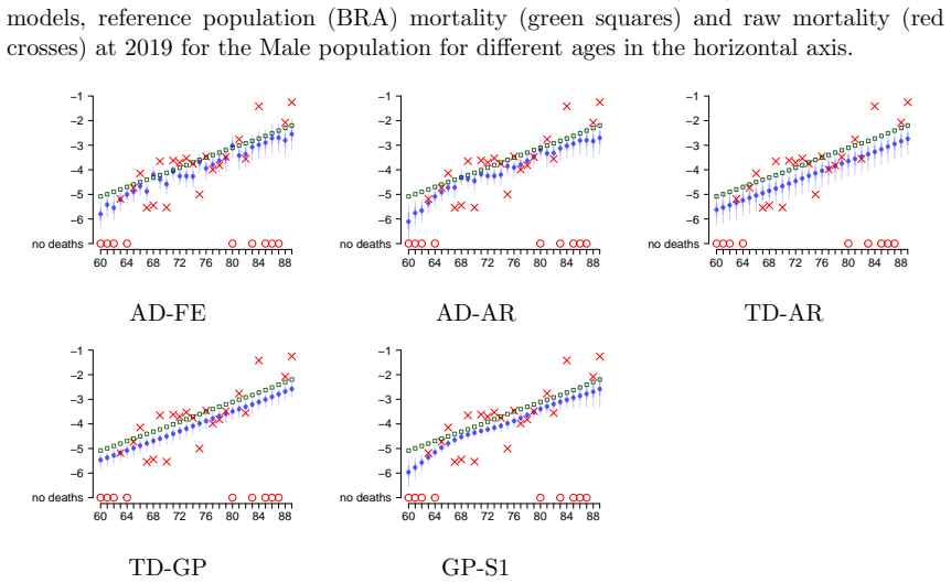
- Because reference-population deflators inherit the reference table's age structure and long-term trend, they avoid the unrealistically steep yearly improvements that a direct bivariate GP (GP-S2) estimates for the fund.
- The estimated overdispersion parameter $\omega$ is consistently above zero, confirming that a Negative Binomial likelihood is needed and that all models agree on the observation error structure.
- Regulatory consistency-test p-values are higher for the AD-GP and GP-S1 models than for the standard AT-2000M annuity table, supporting their use in practice.
Reading between the lines
- If the paper's central claim is right, the same GP-deflator construction should transfer to other sparse sub-populations, including small insurers, regional cohorts, and occupation-specific annuitants, wherever a reliable national or industry reference table exists.
- A testable extension is to propagate uncertainty from the reference table itself: the authors extrapolate the national table's oldest ages with a Gompertz law and interpolate the industry table's publication years with a separate GP, but they do not pass those uncertainties into the deflator posteriors, so a hierarchical version would likely widen predictive intervals.
- One could also extend the deflator GP to a joint age-year surface with a separable kernel; the data here are too sparse to identify both dimensions, but larger sub-populations or longer observation windows would make that specification testable.
- Finally, the framework suggests a practical prior-tuning rule: when observed fund improvements are unsustainably fast, informative priors borrowed from reference-population projections should be used to stabilize long-horizon forecasts, a strategy the paper endorses but does not fully formalize.
Editorial analysis
A structured set of objections, weighed in public.
Referee Report
Summary. The paper develops a family of Bayesian sub-population mortality models for small pension fund populations, in which the fund's mortality is represented through deflators relative to an external reference table (Brazilian national IBGE and insurance-industry BR-EMS tables). The deflators are modeled variously as constant (FD-1), age-dependent fixed effects (AD-FE), autoregressive (AD-AR), Gaussian-process age-dependent (AD-GP), time-dependent (TD-AR, TD-GP), and are compared with direct single-population GP models (GP-S1, GP-S2). All stochastic models use a Negative Binomial likelihood with overdispersion hyperparameter and are fitted in Stan with fully specified priors. The empirical illustration uses male pensioners aged 60–89 from two Brazilian pension funds, with a leave-one-year-out cross-validation over 2013–2019 and predictive scores (log-score, RPS, MAE). The authors claim that GP-based models achieve better goodness of fit and uncertainty quantification than parametric alternatives, and they recommend AD-GP for the primary fund and TD-GP for the second fund.
Significance. If the comparative claims were rigorously established, the paper would be a useful contribution to actuarial mortality modeling for sparse sub-populations: the model taxonomy is well organized, the fully Bayesian implementation with explicit priors and Stan code is a strength, and the two Brazilian case studies provide new empirical evidence on mortality basis risk in a high-inequality setting. The paper also makes a sensible practical point that deflator-based models borrow strength from reference tables. However, the central empirical claim—that GP models outperform parametric alternatives in both fit and uncertainty quantification—is not supported by the reported metrics alone, because the score differences are small, no uncertainty or significance assessment is attached to them, the ranking changes across the two data sets, and the uncertainty quantification is never calibrated. These issues are fixable within the manuscript's scope.
major comments (4)
- [Table 1 and Section 6] The claim that GP models 'achieve better goodness of fit' (abstract) is not statistically substantiated. In Table 1, out-of-sample RPS ranges only from 0.649 to 0.674 and log-score from 1.413 to 1.452; the best model GP-S1 (RPS 0.649) is separated from AD-GP and AD-AR (0.654) by differences that are likely within Monte Carlo or fold-to-fold noise. No standard errors, confidence intervals, or predictive-accuracy tests (e.g., Diebold–Mariano test or bootstrap over the 210 held-out age-year pairs) are reported. The prose also appears internally inconsistent: Section 6 declares GP-S1 the overall winner, while Section 7 recommends AD-GP for pension fund 1 despite its slightly worse Table 1 scores. Please add a formal comparison of predictive scores, or temper the ranking claims accordingly.
- [Section 5.2 and Section 6] The uncertainty-quantification claim is not validated. The text treats narrower posterior intervals as beneficial (Section 5.2, Figure 5), but no calibration check is performed: for example, the empirical coverage of the 50% and 90% predictive intervals for held-out death counts (Figure 6, bottom row) is never computed. Without such checks, 'better uncertainty quantification' is an unsupported assertion. I recommend reporting coverage rates and, if possible, proper scoring rules that explicitly reward calibrated dispersion (e.g., interval scores or quantile coverage plots).
- [Section 3, paragraphs 3–4] The reference tables are treated as known inputs, but they are themselves constructed: IBGE rates for ages 81–89 are extrapolated using a Gompertz model, and BR-EMS rates are interpolated across publication years with a separate GP fit. The uncertainty of these preprocessing steps is not propagated into the deflator posterior or into the forecasts, so any bias in the reference values directly biases every deflator-based estimate. At minimum, the authors should provide a sensitivity analysis (e.g., varying the Gompertz extrapolation or the GP interpolation) and should state clearly in Section 6 that the reported uncertainty intervals condition on the reference table being exact.
- [Appendix C, Table 3] The ranking of models changes materially across the two pension funds. For pension fund 2, TD-GP is best by RPS (0.5147) and log-score (1.2557), while AD-GP (0.5197) is worse than the constant-deflator FD-1 (0.5171) and essentially tied with GP-S1 (0.5185). This contradicts the general statement in Section 7 that 'GP-based models outperform other deflator approaches' and reinforces the concern that the Table 1 differences are within noise. The authors should either provide a combined statistical comparison across both funds or explicitly restrict their comparative claims to the specific data sets analyzed, with appropriate uncertainty.
minor comments (4)
- [Section 5.1] The statement 'we can reject the hypothesis of omega=0 at 95% confidence level' uses a 90% posterior credible interval; this is a Bayesian credible-interval statement, not a frequentist confidence-level rejection. Please rephrase to avoid confusion.
- [Equation (2) and (3)] The squared-exponential kernel is defined without a noise term (nugget). For mortality data with overdispersion this is acceptable because the Negative Binomial likelihood provides observation noise, but the authors should state explicitly that the GP is for the latent log-deflator and that no nugget is used.
- [Section 4.4, priors for GP-S2] In GP-S2, the prior for sigma^2 is listed in Table 2 but the model definition in Section 4.4 does not restate it; please ensure the model block is self-contained or cross-reference Table 2 clearly.
- [Section 3, Figure 3] The caption for Figure 3 says 'ages 60–80' but the text later discusses extrapolation to age 89; please clarify whether the plotted reference tables are truncated at age 80 or include the extrapolated ages.
Circularity Check
No significant circularity: the GP-deflator comparison is an out-of-sample predictive exercise against exogenous reference tables, and the self-citations are not load-bearing.
full rationale
The paper's central result is an empirical comparison of eight models via leave-one-out cross-validation on 2013-2019 pension fund death counts (Section 6, Table 1), with 2019 as a genuine hold-out year (Section 5.5). The GP deflator models estimate latent functions theta from the fund's own d and E data through the likelihood d ~ NegBin(exp(theta) m_ref E); the reference mortality m_ref is an external IBGE or BR-EMS table, not derived from the fund deaths. Thus the 'deflator' identity theta = log m_fund - log m_ref is a reparameterization, not a reduction of the prediction to the input. The only preprocessing that involves a fitted GP is the interpolation of BR-EMS rates across publication years (Section 3), but that GP is fitted to the insurance-industry table, not to the pension fund deaths, and it is not the source of the claimed out-of-sample gains. The paper cites the authors' own earlier GP mortality work (Ludkovski et al. 2018) and multi-output GP work (Huynh and Ludkovski 2021, 2024), but these citations are contextual: the GP machinery here is standard and implemented directly in Stan, the multi-output approach is explicitly not used, and no uniqueness or optimality theorem is imported from those papers to force the model choice. The weaknesses noted by the skeptic (score differences within noise, no coverage checks, reference-table interpolation uncertainty) are correctness and robustness concerns, not circularity. Accordingly no load-bearing step reduces by construction to its own inputs.
Assumptions & free parameters
free parameters (7)
- Overdispersion ω per reference population =
posterior mode ≈ 0.2 (AD-GP, BRA)
- GP process variance σ² =
prior N(0.5, 0.5²), truncated; posterior not reported numerically
- GP lengthscale φ_age =
posterior mean ≈ 5.5 (AD-GP)
- GP lengthscale φ_year =
posterior mean ≈ 5.1 (TD-GP)
- AR persistence ρ =
posterior mean 0.78 (AD-AR)
- Prior mean for log-deflators θ =
-0.5 for all deflator models
- GP-S1/S2 regression coefficients β0, β_age, β_year =
β0 ≈ -5, β_age ≈ 0.1, β_year ≈ -0.078
assumptions (3)
- domain assumption Death counts follow a Negative Binomial distribution with mean e^{θ}·m_ref·E and variance inflated by ω.
- domain assumption The reference mortality tables (IBGE and BR-EMS) are accurate external baselines for the pension fund population, including ages 81-89 extrapolated by a Gompertz model and years between BR-EMS vintages interpolated by a GP.
- domain assumption The true deflator (or log-mortality) is a smooth function of age and/or year, as captured by a squared-exponential Gaussian process.
Cite this review
Pith. "Pith review of Analyzing Pension Fund Mortality with Gaussian Processes in a Sub Population Framework." pith.science (2026). https://pith.science/paper/VLDFTYIA
@misc{pith2026250603584,
  author       = {Pith},
  title        = {Pith review of: Analyzing Pension Fund Mortality with Gaussian Processes in a Sub Population Framework},
  year         = {2026},
  howpublished = {\url{https://pith.science/paper/VLDFTYIA}},
  note         = {Machine review of arXiv:2506.03584}
}
read the original abstract
Pension fund populations often have mortality experiences that are substantially different from the national benchmark. In a motivating case study of Brazilian corporate pension funds, pensioners are observed to have mortality that is 40-55% below the national average, due to the underlying socioeconomic disparities. Direct analysis of a pension fund population is challenging due to very sparse data, with age-specific annual death counts often in low single digits. We design and study a collection of stochastic sub-population frameworks that coherently capture and project pensioner mortality rates via deflator factors relative to a reference population. Superseding parametric approaches, we propose Gaussian process (GP) based models that flexibly estimate Age- and/or Year-specific deflators. We demonstrate that the GP models achieve better goodness of fit and uncertainty quantification. Our models are illustrated on two Brazilian pension funds in the context of exogenous national and insurance industry mortality tables. The GP models are implemented in R Stan using a fully Bayesian approach and take into account over-dispersion relative to the Poisson likelihood.
Figures


Figures from the paper (12 more)




Reference graph
Works this paper leans on
-
[1]
Alexander, M., Zagheni, E., and Barbieri, M. (2017). A flexible B ayesian model for estimating subnational mortality. Demography , 54(6):2025--2041
work page 2017
-
[2]
Bienvenüe, A. and Rulli \'e re, D. (2012). Iterative adjustment of survival functions by composed probability distortions. The Geneva Risk and Insurance Review , 37(2):156--179
work page 2012
-
[3]
Brouhns, N., Denuit, M., and Vermunt, J. K. (2002). A P oisson log-bilinear regression approach to the construction of projected lifetables. Insurance: Mathematics and economics , 31(3):373--393
work page 2002
-
[4]
Cairns, A. J. G., Blake, D.and Dowd, K., Coughlan, G. D., Epstein, D., Ong, A., and Balevich, I. (2009). A quantitative comparison of stochastic mortality models using data from E ngland and W ales and the U nited S tates. North American Actuarial Journal , 13(1):1--35
work page 2009
-
[5]
Carpenter, B., Gelman, A., D.Hoffman, M., Lee, D., Goodrich, B., Betancourt, M., Brubaker, M., Guo, J., Li, P., and Riddell, A. (2017). Stan: a probabilistic programming language. Journal of Statistical Software , 76(1):1--32
work page 2017
-
[6]
Chen, T., Dai, B., Wang, R., and Liu, D. (2014). Gaussian-process-based real-time ground segmentation for autonomous land vehicles. Journal of Intell. Robotic Systems , 76:563–582
work page 2014
-
[7]
Cressie, N. (1990). The origins of kriging. Mathematical Geology , 22:239--252
work page 1990
-
[8]
Czado, C., Gneiting, T., and Held, L. (2009). Predictive model assessment for count data. Biometrics , 65(4):1254--1261
work page 2009
Show all 44 references
-
[9]
J., Blake, D., Coughlan, G
Dowd, K., Cairns, A. J., Blake, D., Coughlan, G. D., and Khalaf-Allah, M. (2011). A gravity model of mortality rates for two related populations. North American Actuarial Journal , 15(2):334--356
2011
-
[10]
Gompertz, B. (1825). On the nature of the function expressive of the law of human mortality, and on a new mode of determining the value of life contingencies. Philosophical transactions of the Royal Society of London , 115:513--583. In a letter to F rancis B aily, E sq
-
[11]
Hardy, M. R. and Panjer, H. H. (1998). A credibility approach to mortality risk. ASTIN Bulletin: The Journal of the IAA , 28(2):269--283
1998
-
[12]
and Onnela, J.-P
Hoffmann, T. and Onnela, J.-P. (2025). gptools: Scalable G aussian P rocess inference with S tan. Journal of Statistical Software , 112:1--31
2025
-
[13]
and Ludkovski, M
Huynh, N. and Ludkovski, M. (2021). Multi-output G aussian P rocesses for multi-population longevity modelling. Annals of Actuarial Science , 15(2):318--345
2021
-
[14]
and Ludkovski, M
Huynh, N. and Ludkovski, M. (2024). Joint models for cause-of-death mortality in multiple populations. Annals of Actuarial Science , 18(1):51--77
2024
-
[15]
J., Booth, H., and Yasmeen, F
Hyndman, R. J., Booth, H., and Yasmeen, F. (2013). Coherent mortality forecasting: the product-ratio method with functional time series models. Demography , 50(1):261--283
2013
-
[16]
IFRS 17 insurance contracts
IASB (2017). IFRS 17 insurance contracts. https://www.ifrs.org/issued-standards/list-of-standards/ifrs-17-insurance-contracts/
2017
-
[17]
Procedimentos para obtenção de uma Tábua Completa de Mortalidade a partir de uma Tábua Abreviada – B rasil 2014
IBGE (2016). Procedimentos para obtenção de uma Tábua Completa de Mortalidade a partir de uma Tábua Abreviada – B rasil 2014 . https://ftp.ibge.gov.br/Tabuas_Completas_de_Mortalidade/Textos_metodologico_e_de_analise/Metodologia_para_transformar_uma_tabua_abreviada_em_completa_...
2016
-
[18]
Complete mortality tables
IBGE (2022). Complete mortality tables . https://www.ibge.gov.br/estatisticas/sociais/populacao/9126-tabuas-completas-de-mortalidade.html?=&t=resultados
2022
-
[19]
Projeções da População: Notas metodológicas 01/2024 B rasil e Unidades da Federação
IBGE (2024). Projeções da População: Notas metodológicas 01/2024 B rasil e Unidades da Federação . https://biblioteca.ibge.gov.br/visualizacao/livros/liv102111.pdf
2024
-
[20]
Lee, R. D. and Carter, L. R. (1992). Modeling and forecasting US mortality. Journal of the American Statistical Association , 87:659--671
1992
-
[21]
and Lu, Y
Li, H. and Lu, Y. (2017). Coherent forecasting of mortality rates: A sparse vector-autoregression approach. ASTIN Bulletin: The Journal of the IAA , 47(2):563--600
2017
-
[22]
Li, J. (2013). A P oisson common factor model for projecting mortality and life expectancy jointly for females and males. Population studies , 67(1):111--126
2013
-
[23]
and Lee, R
Li, N. and Lee, R. (2005). Coherent mortality forecasts for a group of populations: An extension of the L ee- C arter method. Demography , 42(3):575--594
2005
-
[24]
and Guillas, S
Liu, X. and Guillas, S. (2017). Dimension reduction for G aussian P rocess emulation: An application to the influence of bathymetry on tsunami heights. SIAM/ASA Journal of Uncertainty Quantification , 5:787--812
2017
-
[25]
Ludkovski, M., Risk, J., and Zail, H. (2018). Gaussian P rocess models for mortality rates and improvement factors. ASTIN Bulletin: The Journal of the IAA , 48(3):1307--1347
2018
-
[26]
Marrel, A., Iooss, B., Van Dorpe, F., and Volkova, E. (2008). An efficient methodology for modeling complex computer codes with G aussian P rocesses. Computational Statistics and Data Analysis , 52(10):4731--4744
2008
-
[27]
and Kurata, E
Mori, H. and Kurata, E. (2008). Application of G aussian P rocess to wind speed forecasting for wind power generation. In 2008 IEEE International Conference on Sustainable Energy Technologies , pages 956--959
2008
-
[28]
and O'Hagan, A
Oakley, J. and O'Hagan, A. (2002). Bayesian inference for the uncertainty distribution of computer model outputs. Biometrika , 89(4):769--784
2002
-
[29]
OECD Economic Surveys: B razil - Overview
OECD (2018). OECD Economic Surveys: B razil - Overview . https://www.oecd.org/economy/brazil-economic-snapshot/
2018
-
[30]
Oliveira, G., Loschi, R., and Assunção, R. (2021). Bayesian dynamic estimation of mortality schedules in small areas. arXiv:2105.02203
2021 arXiv
-
[31]
Olivieri, A. (2011). Stochastic mortality: experience-based modeling and application issues consistent with S olvency 2. European Actuarial Journal , 1:101--125
2011
-
[32]
and Pitacco, E
Olivieri, A. and Pitacco, E. (2012). Life tables in actuarial models: from the deterministic setting to a B ayesian approach. AStA Advances in Statistical Analysis , 96(2):127--153
2012
-
[33]
Plat, R. (2009). Stochastic portfolio specific mortality and the quantification of mortality basis risk. Insurance: Mathematics and Economics , 45(1):123--132
2009
-
[34]
Rasmussen, C. E. and Williams, C. K. I. (2005). Gaussian Processes for Machine Learning (Adaptive Computation and Machine Learning) . The MIT Press
2005
-
[35]
Renshaw, A. E. and Haberman, S. (2006). A cohort-based extension to the Lee--C arter model for mortality reduction factors. Insurance: Mathematics and economics , 38(3):556--570
2006
-
[36]
and Idier, D
Rohmer, J. and Idier, D. (2012). A meta-modelling strategy to identify the critical offshore conditions for coastal flooding. Natural Hazards and Earth System Sciences , 12:2943--2955
2012
-
[37]
Roustant, O., Ginsbourger, D., and Deville, Y. (2012). DiceKriging, DiceOptim : Two R packages for the analysis of computer experiments by K riging-based metamodeling and optimization. Journal of Statistical Software , 51(1):1--55
2012
-
[38]
and Loisel, S
Salhi, Y. and Loisel, S. (2017). Basis risk modelling: A cointegration-based approach. Statistics , 51(1):205--221
2017
-
[39]
Salhi, Y., Thérond, P., and Tomas, J. (2015). A credibility approach of the M akeham mortality law. European Actuarial Journal , 6(1):61--96
2015
-
[40]
Sandström, A. (2016). Handbook of Solvency for Actuaries and Risk Managers: Theory and Practice . CRC Press
2016
-
[41]
RStan : the R interface to Stan
Stan Development Team (2018). RStan : the R interface to Stan . R package version 2.18.2
2018
-
[42]
and Planchet, F
Tomas, J. and Planchet, F. (2015). Prospective mortality tables: taking heterogeneity into account. Insurance: Mathematics and Economics , 63:169--190
2015
-
[43]
United Nations, U. (2015). Estimating life tables for developing countries. Population Division. Technical Paper No. 2014/4
2015
-
[44]
van Berkum, F., Antonio, K., and Vellekoop, M. (2017). A B ayesian joint model for population and portfolio-specific mortality. ASTIN Bulletin: The Journal of the IAA , 47(3):681--713
2017
Reviewed August 7, 2026 · model on record in the stance chip above.
Discussion (0). Sign in to comment.