REVIEW 2 major objections 4 minor 34 references
Adaptive Grid Designs for Classifying Monotonic Binary Deterministic Computer Simulations
T0 review · 2 major / 4 minor · reviewed 2026-08-07 · deepseek-v4-flash
Pith's one-line read Nested adaptive grids that skip logically forced runs trace a monotone simulator's success–failure boundary at the best possible adaptive rate — about $v^{-(p-1)}$ runs in $p \ge 2$ dimensions, an order of magnitude better than any static…
desk verdict Useful worst-case lower bounds for static and adaptive designs, but the paper's advertised upper bound for the adaptive grid design does not match its own algorithm; the central rate claim is unsupported as printed. read the letter →
The pith
A machine-rendered reading of the paper's core claim, the machinery that carries it, and where it could break.
The reading
What carries the argument
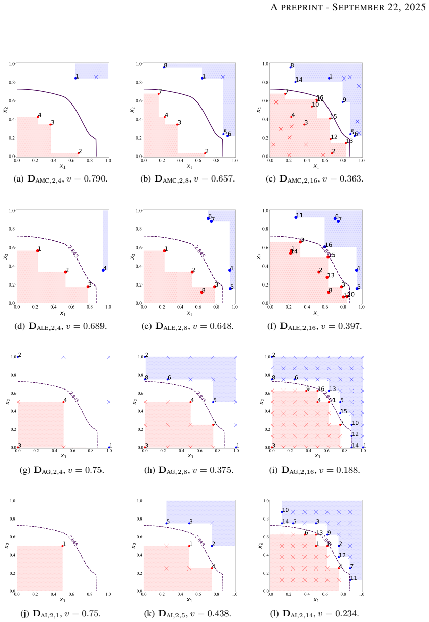
The engine of the method is logical run-skipping under total monotonicity. After a point $x$ is evaluated, the outcome is forced at every point in the lower orthant $[0, x]$ if $f(x) = -1$ and in the upper orthant $[x, 1]$ if $f(x) = 1$, so the uncertain region $U(D, f)$ is the complement of these covered orthants and its volume $V(U)$ is the paper's measure of classification error. The adaptive grid design is a named class of designs: sequences of nested full grids with $(2^l + 1)^p$ points per grid ($3^p, 5^p, 9^p, 17^p, \ldots$), run from coarse to fine, in which only points that fall inside the current uncertain region get evaluated. The grouped variant (GG, Algorithm 1) processes one whole resolution before updating $U$ and carries the proved rate; the fully adaptive variant (AG, Algorithm 2) updates $U$ after every run and chooses next the point that maximizes the number of remaining candidates it will render skippable, $\min\{\mathrm{card}(A_x), \mathrm{card}(B_x)\}$ — numerically stronger, without a matching theorem. The lower bounds are proved by an adversarial monotone threshold function on $\sum_k x_k$ that forces any design with few points to leave thin uncovered slices of the input box, which makes the static and adaptive exponents $n^{-1/p}$ and $n^{-1/(p-1)}$ unavoidable.
What would settle it
Run the ice-breaking finite-element model at pairs of inputs ordered by the paper's reparameterization (higher velocity, lower thickness, lower modulus all push the output up); the first pair with a 'break' at the lower input and a 'no break' at the higher input refutes the monotonicity premise on which the skipping logic and the $V(U)$ guarantee rest. Separately, run the fully adaptive grid method on a known monotone test function with boundary $\sum_k x_k = p/2$ for $p = 2$ and $p = 3$, record the evaluations needed to reach $V(U) \le v$ for $v = 10^{-1}, 10^{-2}, 10^{-3}$, and check that the count grows as $v^{-(p-1)}$ rather than $v^{-p}$.
Extended reading notes
Core claim
The central claim is that the worst-case cost of classifying a monotone binary deterministic simulator is governed by the dimension of the boundary, not of the input space, provided runs may be chosen adaptively. For $p \ge 2$, the volume of the uncertain region $V(U)$ after $n$ runs is at most a constant times $n^{-1/(p-1)}$ for the proposed adaptive grid design (Theorem 3), while no adaptive design can force it below a constant times $n^{-1/(p-1)}$ (Theorem 4) and no static design can beat a constant times $n^{-1/p}$ (Theorems 1 and 2). In terms of runs needed to guarantee $V(U) \le v$, that is order $v^{-(p-1)}$ for the adaptive grid, order $v^{-(p-1)}$ for the best possible adaptive design, and order $v^{-p}$ for the best possible static design — so the adaptive grid is worst-case optimal up to constants among all adaptive procedures and better than any static design by a full power of $1/v$; for $p = 1$ the comparison is $\log(1/v)$ versus $1/v$. The paper's grouped-adaptive grid design carries this rate guarantee; its fully adaptive variant is shown numerically to be even better, and the authors state that they could not prove a matching theorem for it. Applications to a road-crash simulator and an ice-breaking finite-element model, where one run costs about ten hours on 120 cores, confirm the practical gain.
Load-bearing premise
The load-bearing premise is that the simulator's output is exactly monotone — non-decreasing in every input coordinate after reparameterization — so that an unevaluated point's outcome is logically forced by comparisons with evaluated points; in the ice-breaking application this is assumed from domain knowledge, and any small numerical non-monotonicity would let a skipped run be misclassified and would void the $V(U)$ guarantee.
Editorial extensions
If this is right
- In $p \ge 2$ dimensions no static design — grid, Latin hypercube, Monte Carlo, or space-filling — can achieve better than order $v^{-p}$ runs, so the $n^{-1/p}$ static rate is a genuine floor (Theorems 1 and 2).
- No adaptive design of any kind can beat order $v^{-(p-1)}$ runs, and the adaptive grid attains it, so the proposed method is minimax-rate optimal up to constants among all adaptive strategies (Theorems 3 and 4).
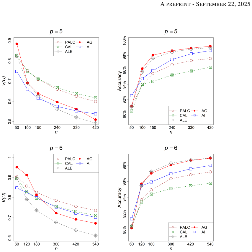
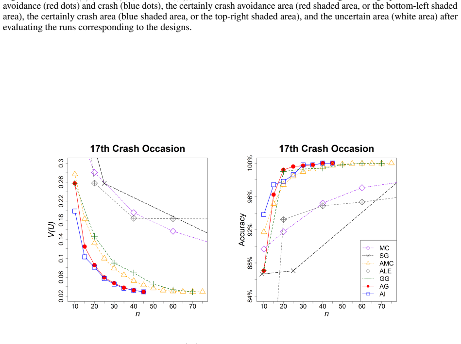
- On the ice-breaking simulator, 29 adaptive grid runs reproduce the uncertainty level of the 125-run static grid — about 12 days of simulation instead of close to two months — and the road-crash results show the same pattern across all 40 reconstructed crash occasions.
- For $p = 1$ the adaptive advantage is exponential: roughly $\log(1/v)$ runs versus order $1/v$ runs for any static design.
- Because all runs in one grid resolution can be evaluated in parallel, the grouped variants (GG, GI) offer a parallel-friendly route, whereas the fully adaptive variants (AG, AI) are sequential but empirically stronger.
Reading between the lines
- Editorial inference: the $v^{-(p-1)}$ rate reads as the cost of locating a $(p-1)$-dimensional boundary to accuracy $v$, whereas static designs pay to resolve the whole $p$-dimensional box; if that geometric reading is right, skipping schemes built on monotone covering should be near-optimal wherever the target is a low-codimension manifold, not only for monotone binary simulators.
- Editorial inference: the same orthant-skipping logic transfers, via the paper's own reparameterizations, to simulators that are monotone decreasing in some coordinates or defined on rectangular domains, and to shape-constrained classification problems beyond deterministic simulation.
- Editorial inference: the paper's numerical comparisons show the grid's edge fading by $p = 6$, where the entropy-based active learning baseline overtakes it, so a hybrid that applies adaptive grids in a few coordinates and entropy acquisition in the rest is a natural, testable next step that the paper does not propose.
- Editorial inference: the lower bounds are driven by adversarial step-shaped boundaries, so on smooth monotone simulators the realized saving over static designs could be larger than the worst-case comparison; a direct measurement on smooth simulators would quantify how much the minimax guarantee understates the practical gain.
Editorial analysis
A structured set of objections, weighed in public.
Referee Report
Summary. The paper studies experimental design for deterministic, binary, monotone computer simulations. It measures design quality by the worst-case volume V(U) of the region whose outcome is not logically forced by the evaluated runs, and it derives lower bounds on the number of runs required by any static design (Theorem 2) and any adaptive design (Theorem 4). It then proposes grouped-adaptive grid (GG) and fully adaptive grid (AG) designs, and proves an upper bound for GG (Theorem 3) that is intended to show that O(v^{-(p-1)}) runs suffice to guarantee V(U)≤v, matching the adaptive lower bound and improving on the static O(v^{-p}) rate. Numerical comparisons on synthetic test functions, road-crash simulation data, and an ice-breaking finite-element simulation demonstrate practical gains for the proposed adaptive grid methods.
Significance. The worst-case rate results are the main contribution. If the intended geometric-grid reading of Theorem 3 is confirmed, the paper provides the first matching-order lower and upper bounds for this class of problems, with a constructive design that is simple to implement and substantially cheaper than static grids. The paper also includes detailed proofs, comparisons with many existing design methods, and two real simulation applications, which strengthen its practical relevance. The main reservation is that the theoretical optimality statement applies to the grouped variant GG, while the fully adaptive variant AG, which is the method recommended for applications, has no supporting theorem; in addition, the grid-level notation in the central upper-bound theorem needs to be made unambiguous.
major comments (2)
- [Section 2.3, Theorem 3, Algorithm 1, Appendix C.3] The grid-level notation must be disambiguated. In the manuscript as reproduced, Algorithm 1 and Theorem 3 state levels with (2l+1) points per dimension, while the proof in Appendix C.3 sets m=2^l and analyzes refinement from m+1 to 2m+1 points per dimension, and the asymptotic sentence after Theorem 3 claims m_GG(g)=O(2^{g(p-1)}). If read arithmetically, the displayed bound sum_{l=1}^g p(2l+1)^{p-1} is O(g^p), so with grid spacing O(1/g) the resulting number of runs is O(v^{-p}), not the claimed O(v^{-(p-1)}); the theorem would then not support the paper's central claim. The surrounding text and proof indicate that the intended construction is geometric, with 2^l+1 points per dimension, in which case the advertised rate follows. Because this is the load-bearing upper bound, the published version must use unambiguous notation throughout and align Algorithm 1, the group definitions, Theorem 3, and the proof; I recommend explicitly writing 2^l+1 rather than 2l+1 and stating the initial level l=0 corresponds to the 2^p corner grid.
- [Abstract, Section 2.3, Section 6] The theoretical optimality result is proved only for the grouped-adaptive grid design GG, not for the fully adaptive grid design AG. Section 2.3 explicitly says that no rigorous theory is established for AG, yet the abstract and conclusions use the phrase 'adaptive grid designs' without qualification when claiming a v^{-(p-1)} evaluation rate that matches the best possible adaptive design. Since AG is the method recommended in the numerical sections and the applications, the paper should either scope the optimality claim to GG or clearly state that the optimality statement is conjectural for AG, so that readers do not attribute a proven rate to the algorithm actually used in practice.
minor comments (4)
- [Appendix C.5, Theorem 5] The displayed limit in Theorem 5 is garbled; it should be lim_{n→∞} E[V{U(D_MC,p,n, f_tilde)}]/n^{-1/p}, not the expression with an extra factor of n in the numerator.
- [Algorithm 1] When l=0, the candidate set is D_SG,p,2^p, the 2^p corner grid. This should be stated explicitly, because a literal reading of '(2l+1)^p' with l=0 would give a degenerate one-point grid that is not covered by the definition of D_SG,p,n.
- [Sections 3-5] The support vector classifier with a Gaussian kernel is not guaranteed to produce monotone predictions. Since the theoretical bounds concern V(U), not classifier accuracy, the paper should clarify that V(U) is the design-efficiency criterion and that the downstream classifier is not assumed to respect monotonicity.
- [Section 5] The ice-breaking application assumes exact monotonicity of the finite-element simulator from domain knowledge. A brief caveat that small numerical non-monotonicities could invalidate the skipping step and hence the V(U) interpretation would be useful, since the paper later says it plans to study violations of the monotonicity assumption.
Circularity Check
No circular derivation: all rate claims are supported by in-paper lower and upper bound proofs from the monotonicity assumption, with no fitted parameter renamed as a prediction and no load-bearing self-citation chain.
full rationale
The central claims do not reduce to their inputs. The worst-case volume of uncertainty is defined directly from the monotonicity assumption, and the upper bound on the grouped-adaptive grid design (Theorem 3) is proved by counting grid points whose outcomes are not forced by monotonic comparisons; no fitted constant enters that count. The lower bounds for static and adaptive designs (Theorems 2 and 4) are proved by explicit adversary constructions, such as threshold functions f_alpha, and are not imported from the authors' prior work or from any citation. The claim that the grouped-adaptive grid design matches the best possible adaptive design is an external comparison of a proved upper bound with a proved lower bound, not a restatement of the algorithm's definition. Numerical sections use independent test functions, the Volvo road-crash dataset, and the ice-breaking simulation as benchmarks; no estimated parameter is subsequently reported as a prediction. The paper contains no self-citation chain that carries a load-bearing premise: references to [24] merely describe the existing adaptive Monte Carlo method, and the road-crash data citation in [4] is external empirical material. There is a genuine internal consistency concern that the proof of Theorem 3 sets m=2l and refines from m+1 to 2m+1 points per dimension, corresponding to geometric grid levels, whereas Algorithm 1 and the theorem statement use arithmetic grid levels with 2l+1 points per dimension; this is a potential proof gap about the advertised v^{-(p-1)} rate, but it is a correctness issue, not a circularity issue, because the derivation is not equivalent to its own conclusion by construction. Under the review rule that most papers are not circular, no circular step is exhibited, so the circularity score is 0.
Assumptions & free parameters
assumptions (4)
- domain assumption The simulation is deterministic and the outcome is exactly binary at every input point.
- domain assumption The response is monotone non-decreasing in every coordinate after linear rescaling.
- ad hoc to paper Worst-case performance, sup over Omega of V(U(D,f)), is the correct efficiency measure.
- ad hoc to paper The candidate grids in Algorithm 1 are nested in the sense needed for the counting proof.
Cite this review
Pith. "Pith review of Adaptive Grid Designs for Classifying Monotonic Binary Deterministic Computer Simulations." pith.science (2026). https://pith.science/paper/PBWYBKQB
@misc{pith2026250603815,
  author       = {Pith},
  title        = {Pith review of: Adaptive Grid Designs for Classifying Monotonic Binary Deterministic Computer Simulations},
  year         = {2026},
  howpublished = {\url{https://pith.science/paper/PBWYBKQB}},
  note         = {Machine review of arXiv:2506.03815}
}
read the original abstract
This research is motivated by the need for effective classification in ice-breaking dynamic simulations, aimed at determining the conditions under which an underwater vehicle will break through the ice. This simulation is extremely time-consuming and yields deterministic, binary, and monotonic outcomes. Detecting the critical edge between the negative-outcome and positive-outcome regions with minimal simulation runs necessitates an efficient experimental design for selecting input values. In this paper, we derive lower bounds on the number of functional evaluations needed to ensure a certain level of classification accuracy for arbitrary static and adaptive designs. We also propose a new class of adaptive designs called adaptive grid designs, which are sequences of grids with increasing resolution such that lower resolution grids are proper subsets of higher resolution grids. By prioritizing simulation runs at lower resolution points and skipping redundant runs, adaptive grid designs require the same order of magnitude of runs as the best possible adaptive design, which is an order of magnitude fewer than the best possible static design. Numerical results across test functions, the road crash simulation and the ice-breaking simulation validate the superiority of adaptive grid designs.
Figures


Figures from the paper (11 more)





Reference graph
Works this paper leans on
-
[1]
Thomas J. Santner, Brian J. Williams, and William I. Notz.The design and analysis of computer experiments. Springer New York, New York, 2003
work page 2003
-
[2]
Qingchen Dong, Wenxin Xue, Taotao Liu, Xin Zhao, and Biao Huang. A numerical simulation method for ice-breaking and cavitation effects on the water-exiting vehicle.Ocean Engineering, 314:119659, 2024
work page 2024
-
[3]
Ying Chen, Jie Li, Zhaoxin Gong, Xin Chen, and Chuanjing Lu. Les investigation on cavitating flow structures and loads of water-exiting submerged vehicles using a uniform filter of octree-based grids.Ocean Engineering, 225:108811, 2021
work page 2021
-
[4]
Henrik Imberg, Xiaomi Yang, Carol Flannagan, and Jonas Bärgman. Active sampling: A machine-learning-assisted framework for finite population inference with optimal subsamples.Technometrics, 0(0):1–12, 2024
work page 2024
-
[5]
Jiakun Zhang, Liang Hao, Qin Wu, and Biao Huang. Numerical investigation on the formation of the re-entrant flow and the transformation of varying shedding modes in cloud cavitation.Ocean Engineering, 279:114557, 2023
work page 2023
-
[6]
Zhuan-Tao He, Chun-Mei Wu, Jia jia Yu, and You-Rong Li. Dynamic analysis of adsorbate behavior in nanopores: Liquid bridge formation, cavitation, and contact angle evaluation via molecular dynamics simulations.Journal of Molecular Liquids, 414:126146, 2024
work page 2024
-
[7]
John Stufken and Min Yang.Optimal designs for generalized linear models, chapter 4, pages 137–164. John Wiley & Sons, Ltd, 2012
work page 2012
-
[8]
Mervyn J. Silvapulle. On the existence of maximum likelihood estimators for the binomial response models. Journal of the Royal Statistical Society: Series B (Methodological), 43(3):310–313, 1981
work page 1981
Show all 34 references
-
[9]
Golchi, D
S. Golchi, D. R. Bingham, H. Chipman, and D. A. Campbell. Monotone emulation of computer experiments. SIAM/ASA Journal on Uncertainty Quantification, 3(1):370–392, 2015
2015
-
[10]
Xiaojing Wang and James O. Berger. Estimating shape constrained functions using gaussian processes.SIAM/ASA Journal on Uncertainty Quantification, 4(1):1–25, 2016
2016
-
[11]
Shape-constrained statistical inference.Annual Review of Statistics and Its Application, 11(V olume 11, 2024):373–391, 2024
Lutz Dümbgen. Shape-constrained statistical inference.Annual Review of Statistics and Its Application, 11(V olume 11, 2024):373–391, 2024
2024
-
[12]
Chih-Li Sung, Ying Hung, William Rittase, Cheng Zhu, and C. F. Jeff Wu. A generalized gaussian process model for computer experiments with binary time series.Journal of the American Statistical Association, 115(530):945–956, 2020
2020
-
[13]
Monotonic random forest with an ensemble pruning mechanism based on the degree of monotonicity.New Generation Computing, 33(4):367–388, 2015
Sergio González, Francisco Herrera, and Salvador García. Monotonic random forest with an ensemble pruning mechanism based on the degree of monotonicity.New Generation Computing, 33(4):367–388, 2015
2015
-
[14]
Xgboost: A scalable tree boosting system
Tianqi Chen and Carlos Guestrin. Xgboost: A scalable tree boosting system. InProceedings of the 22nd ACM SIGKDD International Conference on Knowledge Discovery and Data Mining, page 785–794. Association for Computing Machinery, 2016
2016
-
[15]
Monotonic classification: An overview on algorithms, performance measures and data sets.Neurocomputing, 341:168–182, 2019
José-Ramón Cano, Pedro Antonio Gutiérrez, Bartosz Krawczyk, Michał Wo´ zniak, and Salvador García. Monotonic classification: An overview on algorithms, performance measures and data sets.Neurocomputing, 341:168–182, 2019
2019
-
[16]
Support-vector networks.Machine Learning, 20(3):273–297, 1995
Corinna Cortes and Vladimir Vapnik. Support-vector networks.Machine Learning, 20(3):273–297, 1995
1995
-
[17]
A comprehensive survey on support vector machine classification: Applications, challenges and trends.Neurocomputing, 408:189–215, 2020
Jair Cervantes, Farid Garcia-Lamont, Lisbeth Rodríguez-Mazahua, and Asdrubal Lopez. A comprehensive survey on support vector machine classification: Applications, challenges and trends.Neurocomputing, 408:189–215, 2020
2020
-
[18]
M. D. McKay, R. J. Beckman, and W. J. Conover. Comparison of three methods for selecting values of input variables in the analysis of output from a computer code.Technometrics, 21(2):239–245, 1979. 35 APREPRINT- SEPTEMBER22, 2025
1979
-
[19]
Myers, and William A
Shan Ba, William R. Myers, and William A. Brenneman. Optimal sliced latin hypercube designs.Technometrics, 57(4):479–487, 2015
2015
-
[20]
Probal Chaudhuri and Per A. Mykland. Nonlinear experiments: optimal design and inference based on likelihood. Journal of the American Statistical Association, 88(422):538–546, 1993
1993
-
[21]
Optimal designs for two-level factorial experiments with binary response.Statistica Sinica, 22(2):885–907, 2012
Jie Yang, Abhyuday Mandal, and Dibyen Majumdar. Optimal designs for two-level factorial experiments with binary response.Statistica Sinica, 22(2):885–907, 2012
2012
-
[22]
Jones, Matthias Schonlau, and William J
Donald R. Jones, Matthias Schonlau, and William J. Welch. Efficient global optimization of expensive black-box functions.Journal of Global Optimization, 13(4):455–492, Dec 1998
1998
-
[23]
Partitioned active learning for heterogeneous systems.Journal of Computing and Information Science in Engineering, 23(4):041009, 01 2023
Cheolhei Lee, Kaiwen Wang, Jianguo Wu, Wenjun Cai, and Xiaowei Yue. Partitioned active learning for heterogeneous systems.Journal of Computing and Information Science in Engineering, 23(4):041009, 01 2023
2023
-
[24]
de Rocquigny
E. de Rocquigny. Structural reliability under monotony: Properties of form, simulation or response surface methods and a new class of monotonous reliability methods (mrm).Structural Safety, 31(5):363–374, 2009
2009
-
[25]
Roshan Joseph, Tirthankar Dasgupta, Rui Tuo, and C
V . Roshan Joseph, Tirthankar Dasgupta, Rui Tuo, and C. F. Jeff Wu. Sequential exploration of complex surfaces using minimum energy designs.Technometrics, 57(1):64–74, 2015
2015
-
[26]
Lewis and William A
David D. Lewis and William A. Gale. A sequential algorithm for training text classifiers. InProceedings of the 17th Annual International ACM SIGIR Conference on Research and Development in Information Retrieval, pages 3–12, London, 1994. Springer London
1994
-
[27]
Active learning by acquiring contrastive examples
Katerina Margatina, Giorgos Vernikos, Loïc Barrault, and Nikolaos Aletras. Active learning by acquiring contrastive examples. InProceedings of the 2021 Conference on Empirical Methods in Natural Language Processing, pages 650–663, Online and Punta Cana, Dominican Republic, Nov...
2021
-
[28]
Active learning query strategies for classification, rgression, and clustering: A survey.Journal of Computer Science and Technology, 35(4):913–945, Jul 2020
Punit Kumar and Atul Gupta. Active learning query strategies for classification, rgression, and clustering: A survey.Journal of Computer Science and Technology, 35(4):913–945, Jul 2020
2020
-
[29]
Support vector machine active learning with applications to text classification
Simon Tong and Daphne Koller. Support vector machine active learning with applications to text classification. Journal of Machine Learning Research, 2:45–66, March 2001
2001
-
[30]
Safety assessment and a parametric study of forward collision-avoidance assist based on real-world crash simulations.Journal of Advanced Transportation, 2021:1–24, 2021
MohammadReza Seyedi, MohammadReza Koloushani, Sungmoon Jung, and Arda Vanli. Safety assessment and a parametric study of forward collision-avoidance assist based on real-world crash simulations.Journal of Advanced Transportation, 2021:1–24, 2021
2021
-
[31]
Collision warning with auto brake: A real-life safety perspective
Erik Coelingh, Lotta Jakobsson, Henrik Lind, and Magdalena Lindman. Collision warning with auto brake: A real-life safety perspective. Inthe 20th International Technical Conference on the Enhanced Safety of Vehicles. National Highway Traffic Safety Administration, 2007
2007
-
[32]
John C. Platt. Probabilities for sv machines. InAdvances in Large-Margin Classifiers. The MIT Press, 09 2000
2000
-
[33]
Computational aspects of three-term recurrence relations.SIAM Review, 9(1):24–82, 1967
Walter Gautschi. Computational aspects of three-term recurrence relations.SIAM Review, 9(1):24–82, 1967
1967
-
[34]
Princeton University Press, New Jersey, 2003
Julian Havil.Gamma: exploring Euler’s constant. Princeton University Press, New Jersey, 2003. 36
2003
Reviewed August 7, 2026 · model on record in the stance chip above.
Discussion (0). Sign in to comment.