Deep Neural Networks Hunting Ultra-Light Dark Matter

Diana L\'opez Nacir; Federico R. Urban; Pavel K\r{u}s

REVIEW 4 major objections 8 minor 1 cited by

Deep Neural Networks Hunting Ultra-Light Dark Matter

T0 review · 4 major / 8 minor · reviewed 2026-08-07 · deepseek-v4-flash

Challenge this review Re-run · record.json Download PDF Read on arXiv ↗

Pith's one-line read Neural networks can detect ultra-light dark matter signals in simulated binary-pulsar timing data, and can tell four particle models apart, the paper argues.

desk verdict A careful ML proof-of-concept for ULDM searches in binary pulsar data, but the sensitivity curves omit the dominant low-mass observable (Ψ′) and the abstract oversells the result. read the letter →

arxiv 2506.04100 v2 pith:6DCWY5BI submitted 2025-06-04 astro-ph.HE astro-ph.CO

Pavel Kůs , Diana López Nacir , Federico R. Urban This is my paper

classification astro-ph.HEastro-ph.CO

keywords ultra-lightdarkmatterpulsartimingbinarypulsarsdeepneuralnetworksautoencoderconvolutionalanomalydetectioncouplingconstraints

verification ladder T0 review T1 audit T2 compute T3 formal

The pith

A machine-rendered reading of the paper's core claim, the machinery that carries it, and where it could break.

The reading

This paper tries to establish that deep neural networks can act as a general-purpose detector of ultra-light dark matter (ULDM) in binary-pulsar timing residuals. It simulates residuals for a low-eccentricity pulsar and shows that an autoencoder, a binary convolutional classifier, and a multiclass convolutional classifier can all flag ULDM signals generated by linear scalar, quadratic scalar, vector, and tensor fields. The networks convert their detection thresholds into coupling-constant sensitivity curves across $10^{-23}$ to $10^{-18}\,\mathrm{eV}$, and the multiclass network can identify which of the four models produced a signal. In the linear scalar case the paper reports ML sensitivities up to roughly an order of magnitude weaker than its one-step Bayesian benchmark, and the main payoff is coverage: the ML tools extend easily to vector and tensor models where the fuller Bayesian pipeline has not been built. The central claim is a proof of concept that data-driven searches can cover the full ULDM model space now, at the price of some sensitivity.

What carries the argument

Two pieces carry the argument. The first is the dimensionless signal strength $S = \|\vec R_{\rm binary,DM}\| / \epsilon$, where $\vec R_{\rm binary,DM}$ is the ULDM-induced part of the timing residuals built from oscillations of the projected semi-major axis $x$ and the Laplace--Lagrange parameters $\eta$ and $\kappa$, and $\epsilon$ is the timing-noise amplitude. Because the residuals are linear in the coupling $\lambda$, the sensitivity limit takes the same form in both methods, $|\lambda_c| = S_c \, \epsilon / \|\vec R_{\rm binary,DM}(\lambda=1)\|$, so the entire ML problem reduces to estimating the critical threshold $S_c$ with a network. The second piece is the architecture set: a convolutional autoencoder trained only on noise that flags high reconstruction error, a binary CNN that separates noise from signal, and a five-way softmax CNN that assigns signals to one of the four ULDM models or to noise, both trained with curriculum learning that starts from strong injections and works down to weak ones.

What would settle it

Generate mock residuals for PSR J1909-3744 with ULDM injections that include the full set of varying orbital elements—in particular the orbital phase $\Psi'$ that the paper's footnote lists as dominant below about $2\times 10^{-20}$ eV—and feed them to the same networks. If the detection thresholds $S_{99}$ at low masses do not drop substantially relative to the three-element curves, the omission would be harmless; if the networks miss injected signals that the full-element signal-to-noise calculation says should be detected, the reported coupling limits would be demonstrably incomplete.

Watch

Extended reading notes

Core claim

On its own terms, the paper's central discovery is that the ULDM imprint on orbital elements leaves enough texture in simulated pulsar residuals for three different neural architectures to recover it, and that the recovered detection threshold can be mapped to a physical coupling constant by a model-independent ratio identity. For spin-0 linear coupling the paper compares this threshold with the one-step Bayesian benchmark and finds the ML curves higher by a factor of order one to ten; the abstract summarises this as comparable sensitivity, while the body quantifies the loss as up to an order of magnitude. For spin-1 and spin-2 ULDM no full Bayesian sensitivity curve exists, and the paper presents the ML curves as the first coupling constraints spanning the full mass range for those models. The multiclass classifier is shown to separate the four signal types from noise and from each other with high accuracy at sufficiently large signal strength. The paper therefore claims a new application, not a new physics mechanism: the ULDM perturbations come from existing post-Keplerian calculations, and the contribution is showing that neural networks can learn that physics from time-series data alone.

Load-bearing premise

The load-bearing premise is that tracking only three orbital elements—the projected semi-major axis and the two Laplace–Lagrange parameters—captures the ULDM signal; the paper's own footnote states that for low-eccentricity systems at masses from about $10^{-23}$ to $2\times 10^{-20}$ eV the dominant sensitivity actually comes from a different, omitted orbital-phase variation, so if that phase variation is important the reported sensitivity curves do not represent the full constraining power of the binary system.

Editorial extensions

If this is right

The same autoencoder and CNN pipelines can place coupling limits on all four ULDM models across $10^{-23}$ to $10^{-18}\,\mathrm{eV}$, including spin-1 and spin-2 models for which no full Bayesian sensitivity curve exists.
A detection candidate strong enough to pass the multiclass network's threshold can be assigned to a specific ULDM spin and coupling type from the residual shape alone, since the five-way classifier separates all models from noise and from each other at high accuracy.
The measured scaling of ML sensitivity with data size, roughly $|\lambda| \sim N^{-0.15}$ to $N^{-0.32}$, is slower than the Bayesian $N^{-1/2}$, so collecting longer or denser timing data will help both methods but should not by itself eliminate the ML sensitivity gap.
The autoencoder's unsupervised mode provides a template-free search: it flags anomalous residuals without being trained on any ULDM signal, which is suited to model-agnostic monitoring once real timing data are used.

Reading between the lines

Editorial extensions of the paper, not claims the author makes directly.

Because only three orbital elements are tracked and the omitted phase variation is acknowledged as dominant below about $2\times 10^{-20}\,\mathrm{eV}$, a plausible reading is that the reported $\lambda_c(m)$ curves are conservative at low mass; adding that phase variation to the network inputs could sharpen the curves and narrow the reported gap to the Bayesian benchmark.
The same architectures could be trained on irregularly sampled real arrival times rather than uniform mock cadences; the convolutional layers would need adaptation, and the comparison would test whether uniform sampling hides part of the sensitivity loss seen with complex noise.
The multiclass confusion matrix could be repurposed as a model-discrimination statistic between ULDM theories, quantifying how often one spin model masquerades as another at moderate signal strength.
Combining several binary pulsars into one input tensor would multiply the effective data volume and could partially compensate for the unfavourable $N$ scaling without demanding better per-pulsar sensitivity.

Share X Bluesky LinkedIn Reddit HN

Editorial analysis

A structured set of objections, weighed in public.

Desk editor's note, referee report, and a circularity audit.

Desk Editor's Note

read the letter

Quick take: this is a genuine proof of concept—clean injection-recovery tests, public code, and the first ML treatment of four ULDM models in binary pulsar timing—but the sensitivity curves are built from a reduced residual model that omits Ψ′, the orbital-phase variation the authors themselves identify as dominant for low-eccentricity binaries over most of the mass range. The stress-test note holds up; this is not a manufactured flaw.

What is new: adapting autoencoder and CNN detectors from GW searches to ULDM in pulsar timing residuals; extending to linear scalar, quadratic scalar, vector, and tensor models; and a multiclass classifier that can distinguish the four signal types. The training/test separation is careful, the noise models (white, white+red, with nuisance parameters) are controlled, and the code is available. The scaling analysis is an honest negative result: with N the ML sensitivity improves roughly as N^{-0.15} to N^{-0.32}, noticeably worse than the Bayesian N^{-0.5}. That alone is useful for anyone thinking about ML searches in this area.

The soft spots are real and load-bearing. First, Eq. (9) contains only δx, δη, δκ; footnote 3 says low-eccentricity systems are most sensitive to Ψ′ for m between 10^{-23} and roughly 2×10^{-20} eV—five of the six decades the paper claims. So the λ_c(m) curves are upper limits within a truncated signal model, not full binary-pulsar constraints. The one-step Bayesian benchmark uses the same truncated residual vector, so the ML-vs-Bayesian comparison is internal to that reduced model. The abstract says sensitivity is comparable; the body reports a factor of 6–10 worse. That mismatch should have been caught. Second, there are no error bars on S99 or λ_c(m); the autoencoder uses two realizations, the CNNs single runs, so it is hard to know how robust the curves are. Third, the multiclass demonstration is at one mass only; fine as an illustration, but not a systematic result. The paper is honest about the Ψ′ issue in the Outlook, where it says including other orbital parameters can boost sensitivity, which is exactly the right warning—but it undercuts the full-mass-range claim in the abstract and introduction.

Who is this for? Someone working on ML methods for pulsar-timing searches, or on ULDM detection strategies, will find it a useful methods paper despite the limitations. It deserves a serious referee, not a desk rejection. A referee should ask for the abstract to match the body, for the Ψ′ omission to be either fixed or made central to a reframed proof-of-concept claim, and for uncertainties on the sensitivity curves. With those, it is publishable.

Referee Report

4 major / 8 minor

Summary. The paper presents a proof-of-concept study applying three machine-learning architectures (a convolutional autoencoder, a binary CNN classifier, and a multiclass CNN classifier) to simulated binary-pulsar timing residuals containing signals from four ultra-light dark matter (ULDM) models: linearly coupled scalar, quadratically coupled scalar, vector, and tensor. The authors generate mock residuals for the low-eccentricity pulsar PSR J1909-3744, train the networks on simulated noise (white, white-plus-nuisance, and white-plus-red noise), and use injection-recovery simulations to derive sensitivity curves for the ULDM coupling constant λ as a function of mass in the range 10^-23 eV to 10^-18 eV. They compare these ML sensitivities with a semi-analytical one-step Bayesian benchmark from their earlier work and report that the ML methods are factors of O(1-10) less sensitive. The multiclass classifier is shown to distinguish the four signal types from each other and from pure noise at a single mass. The central claims are that ML provides a practical route to ULDM searches for vector and tensor models where the full Bayesian method has not been implemented, and that the ML sensitivity is 'comparable' to the Bayesian approach.

Significance. If the sensitivity estimates were physically complete, this would be a useful contribution: it would extend ULDM searches to spin-1 and spin-2 models using a reproducible ML pipeline, with public code, controlled injection-recovery tests, separated training and test sets, and a multiclass classifier that can discriminate between signal models. These are real strengths. However, the physical completeness of the sensitivity estimates is the central issue. The residual model in Eq. (9) tracks only δx, δη, and δκ, while the authors' own footnote 3 states that the dominant low-mass observable is the orbital-phase variation Ψ′, which is not included. As a result, the reported λ_c(m) curves are not full binary-pulsar constraints in five of the six decades claimed. The abstract also overstates the comparison with the Bayesian benchmark: the body reports a factor of 6-10 worse sensitivity, not 'comparable'. These issues affect the paper's headline claims, so the significance is currently conditional on substantial revision.

major comments (4)

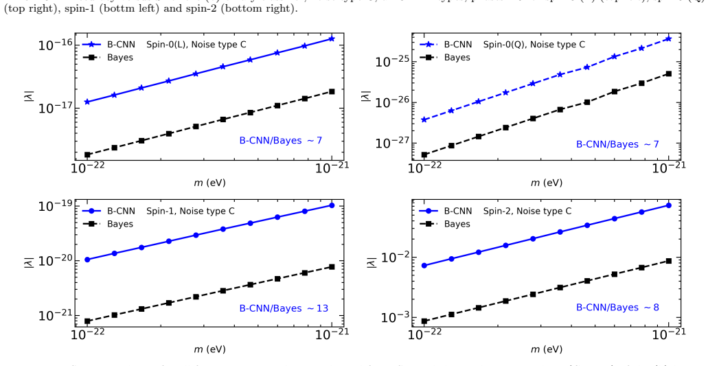
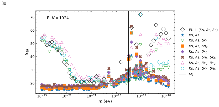
[Section 2.1.5, Eq. (9), footnote 3; Figs. 10, 11, 14, 17] The sensitivity curves are derived from a residual model that omits the dominant low-mass signal. Footnote 3 states that for low-eccentricity binaries in the mass range 10^-23 eV to ~2×10^-20 eV, the dominant ULDM effect is the variation of the orbital phase Ψ′ = ∫ω_b dt′, which is not included in Eq. (9). Since Eq. (9) is the only signal model used to define S (Eq. (54)) and hence λ_c (Eq. (55)), the S99 and λ_c(m) curves in Figs. 10, 11, 14, and 17 characterize sensitivity only to δx, δη, and δκ. In the mass range where the omitted phase variation dominates, these curves are inflated upper limits on λ_c rather than full binary-pulsar constraints. The Conclusion's claim that the ML methods 'place constraints on the ULDM coupling constant across the entire mass range' is therefore not supported. The Outlook (Section 5) acknowledges that including other orbital parameter variations can significantly boost sensitivity at least for the spin-0 linear coupling case, which confirms that the omission is material rather than cosmetic.
[Abstract versus Sections 3.8.3, 3.9.3, 4, and 5] The abstract claims that the sensitivity achieved with ML methods is 'comparable' to the semi-analytical Bayesian approach, but the body reports a consistent factor-of-6-10 gap: Section 3.9.3 states the CNN sensitivity is lower than the Bayesian line by a factor of ~6, Section 3.8.3 reports autoencoder curves above the Bayesian ones by O(1) to O(10), and Section 4 and Section 5 summarize the gap as O(1-10). This is a substantial discrepancy between the abstract and the quantitative results. The abstract should be revised to state the actual factors or to qualify the claim explicitly.
[Figs. 10, 11, 14, 17 and Section 4 scaling fits] The sensitivity curves and the scaling-law fits are presented as single curves without statistical uncertainties. The only randomness accounted for is two noise realizations for the autoencoder (Section 3.8.2), and the CNN training uses stochastic optimization and limited dataset sizes (e.g., 3,000 time series per S value in Section 3.9.2). Because the comparison with the Bayesian benchmark hinges on factors of ~6-10, the absence of error bars or repeated-seed/bootstrapped confidence intervals makes it impossible to assess whether the reported differences between ML and Bayesian sensitivities, or the differences between noise types, are statistically significant. Please add at least a few independent training seeds or a bootstrap over test sets for the headline curves.
[Section 3.4, Eq. (56)] The Bayesian benchmark used for comparison is the simplified one-step approach with delta-function priors, not the two-step Bayesian method of Kus et al. (2024) that is described in the Introduction as the reference method. Moreover, this benchmark is computed from the same truncated residual model in Eq. (9), so the comparison is internal to the reduced (δx, δη, δκ) signal space. The claim that ML sensitivity is 'comparable' to a Bayesian approach therefore refers only to the sensitivity of the truncated model and cannot be read as a statement about the full physical signal or about the two-step method. This limitation should be stated explicitly wherever the comparison is summarized.

minor comments (8)

[Section 3.8.3] The sentence 'We will discuss of the strong mass dependence of S99 in Section 4' should read 'We will discuss the strong mass dependence of S99 in Section 4.'
[Fig. 12 caption] The caption reads 'Same af Fig. 11' and should be 'Same as Fig. 11.'
[Figs. 16 and 17 captions] The captions contain 'bottm left' and should read 'bottom left.'
[Section 3.9.2] The phrase 'training the and binary classifiers' appears to be missing a word; please revise to 'training the autoencoder and binary classifiers' or similar.
[Eq. (54)] The notation \vec{R}^{\mathrm{binary,DM}} is used without an explicit definition of the vector components; please define the vector and its squared norm consistently with Eq. (9), where the individual residual components are written as R^{\mathrm{binary}}_a.
[Table 1] Table 1 lists both ω_b = 4.1 day^{-1} and ω_b = 3.1 × 10^{-20} eV; please clarify that these are the same quantity expressed in different units.
[References] Several references have incomplete author lists (e.g., 'Jing Luo et al.', 'Tarafdar Pratik et al.', 'Zic Andrew et al.'); please format them consistently with the journal style.
[Section 3.10.2 and Section 5] The multiclass classifier is trained only at a single mass, m = 10^{-21} eV, and with noise of type C. The conclusion should explicitly state that the model-discrimination result is a single-mass proof of concept, not a demonstrated capability across the full mass range.

Circularity Check

0 steps flagged · score 2.0 of 10

No significant circularity: ML sensitivities are measured by injection-recovery, and the Bayesian comparison is transparent via in-text Eqs. (55)-(56); the acknowledged Psi-prime omission is a completeness issue, not a circular reduction, and the benchmark self-citation is minor.

full rationale

The central claim is established by measurement, not by derivation from the target: the autoencoder is trained on noise-only data, the CNNs are trained on injected signals, and S99 thresholds are read off accuracy curves and converted to coupling limits through the linear scaling in Eq. (55). No fitted parameter is renamed as a prediction, and the sensitivity curves are not statistically forced by their own inputs. The Bayesian comparison is fully transparent: Eqs. (55) and (56) share the identical template norm in the denominator and differ only by the scalar factor Sc versus sqrt(ln B) = 2.63, exactly as the paper states; Eq. (56) is reproduced in-text as a closed-form formula, so the comparison does not reduce to an unverifiable self-citation. The citation to the authors' Kus et al. (2024) supports only ancillary assertions (that the one-step benchmark tracks the two-step method, and the Psi-prime dominance claim), which is a minor, non-load-bearing self-citation. Two in-paper admissions are weighed here as non-circular. Footnote 3 states that for low-eccentricity systems in the range 10^-23 eV to ~2x10^-20 eV (five of the six claimed decades) the dominant observable is the orbital-phase variation Psi-prime, which is absent from Eq. (9), and the Outlook repeats that including other orbital-parameter variations 'can significantly boost sensitivity, at least for the spin-0 linear coupling case'; this makes the reported lambda_c(m) curves partial estimates rather than full constraints - a completeness/correctness concern, not a circular reduction, because the curves are measured rather than constructed to equal their inputs. The abstract/body mismatch ('comparable' versus factor 6-10 worse in the body) is a wording inconsistency, likewise not circularity. Overall, no step in the derivation chain is equivalent by definition to its input; one minor non-load-bearing self-citation keeps the score at 2.

Assumptions & free parameters 5 free parameters · 6 assumptions · 0 invented entities

The central claim rests on standard ULDM field descriptions and noise models from prior literature (much of it self-cited), plus explicit simplifications: three orbital parameters, fixed fiducial configurations, and Gaussian noise. No new particles, forces, or entities are postulated.

free parameters (5)

Fiducial ULDM configuration parameters = rho=0.707, Upsilon=45 deg (spin-0); spin-1 adds theta=phi=60 deg; spin-2 adds chi=60 deg, epsS=epsT=0.707
Chosen by hand in Section 3.3 to evaluate Eq. (55); the reported lambda_c(m) curves are conditional on these values and would shift under other choices.
Detection threshold and accuracy quantiles = 0.99 quantile of normal reconstruction error; 99% required detection rate for S99
Defines the critical signal strength S99 in Section 3.8.3; changing these changes lambda_c.
Bayes factor B = 1000
Sets sqrt(ln B) approx 2.63 in Eq. (56) for the one-step Bayesian benchmark.
Curriculum learning schedule = initial S=25 to 13 (binary), S=35 to 11 (all-model), S=30 to 18 (multiclass), step 3
Hand-chosen training schedule in Sections 3.9.2 and 3.10.2; affects the achieved sensitivity and the false-positive rate.
Network architectures and hyperparameters = conv filters, kernel sizes, learning rate 0.001, dropout rates, etc.
Selected after limited tuning (Sections 3.7-3.10); affect detection accuracy and the resulting sensitivity curves.

assumptions (6)

domain assumption ULDM is a classical oscillating field with Rayleigh-distributed amplitude and random phase, coherent over the observation time
Used in Section 2.2.1 to generate signal injections; standard in ULDM literature.
domain assumption Signal templates for linear scalar, quadratic scalar, vector, and tensor ULDM from Blas et al. 2017/2020, Lopez Nacir and Urban 2018, and Armaleo et al. 2020
Inputs generated from prior works by the same group; the paper does not re-derive them.
domain assumption Timing residuals follow Gaussian white and/or Lorentzian red noise with the specified covariance matrices
Section 2.1.2; used for both training and evaluation.
ad hoc to paper The ELL1 binary model with low eccentricity and only three tracked orbital parameters (a, eta, kappa) is sufficient for the proof of concept
Section 2.1.5 and footnote 3; the paper acknowledges that the most sensitive parameter Psi' is omitted.
ad hoc to paper Fiducial ULDM configuration values are fixed for each model
Section 3.3; sensitivity is conditional on these choices, not marginalized.
standard math One-step Bayesian method with delta-function priors from Kus et al. 2024 is a valid benchmark
Section 3.4; from the authors' prior paper, used as the comparison standard.

how reviews work

0 comments

Cite this review

Pith. "Pith review of Deep Neural Networks Hunting Ultra-Light Dark Matter." pith.science (2026). https://pith.science/paper/6DCWY5BI

@misc{pith2026250604100,
  author       = {Pith},
  title        = {Pith review of: Deep Neural Networks Hunting Ultra-Light Dark Matter},
  year         = {2026},
  howpublished = {\url{https://pith.science/paper/6DCWY5BI}},
  note         = {Machine review of arXiv:2506.04100}
}

read the original abstract

Ultra-light dark matter (ULDM) is a compelling candidate for cosmological dark matter. If ULDM interacts with ordinary matter, it can induce measurable, characteristic signals in pulsar-timing data because it causes the orbits of pulsars in binary systems to osculate. In this work, we investigate the potential of machine learning (ML) techniques to detect such ULDM signals. To this end, we construct three types of neural networks: an autoencoder, a binary classifier, and a multiclass classifier. We apply these methods to four theoretically well-motivated ULDM models: a linearly coupled scalar field, a quadratically coupled scalar field, a vector field and a tensor field. We show that the sensitivity achieved using ML methods is comparable to that of a semi-analytical Bayesian approach, which to date has only been applied to the linear scalar case. The ML approach is readily applicable to all four ULDM models and, in the case of the multiclass classifier, can distinguish between them. Our results, derived from simulated data, lay the foundation for future applications to real pulsar-timing observations.

Figures

Figures reproduced from arXiv: 2506.04100 by the authors.

**Figure 1.** — Illustration of a binary pulsar inside a dark matter halo that follows a non-Keplerian orbit caused by interaction with ULDM. Although the gravitational imprint on pulsar timing data appears too weak to be detectable (Blas et al. 2020), a signal from direct ULDM-matter interaction could be observed. If such a signal is not detected, it would place stringent constraints on the ULDM parameter space. Initial studies … view at source ↗

**Figure 2.** — Left panel: Examples of time residuals for white noise, red noise and an equally weighted combination of white and red noise. These apply to the low-eccentricity pulsar PSR J1909-3744, with N = 1024 uniformly distributed data points. Right panel: Power spectral densities for the same simulated data. PG stands for periodogram, T stands for theory prediction. TABLE 1 Parameters for PSR J1909-3744 (Agazie et al. 2023… view at source ↗

**Figure 3.** — Description of Keplerian orbits in terms of the orbital elements viewed in the fundamental reference frame (X, Y, Z). The Cartesian orbital frame (x, y, z) and the polar one (r, θ, z) are also shown (centred on M2 for convenience). 2.1.4. Binary system description In an idealised binary system stars follow elliptical orbits described by six orbital parameters. Two of these parameters define the shape and size of … view at source ↗

Figures from the paper (25 more)

**Figure 4.** Figure 4: — Binary systems are located in distinct ULDM patches, each approximately λdB/2 in size. ULDM is not a single theory but rather a class of models. We consider four viable ULDM models: (pseudo)scalar fields with linear or quadratic direct couplings to ordinary matter vi…

**Figure 5.** Figure 5: — Distribution on the sphere of 200 red (blue) points when using the Gaussian (direct) sampling approach. For the spin-2 ULDM field, the configuration is parametrised by three real numbers, ϵS, ϵV and ϵT , which satisfy the normalisation condition, along with two angul…

**Figure 6.** Figure 6: illustrates the contributions of each signal type and how they combine to form complex time residuals. Specifically, the top and middle panels show the contributions of individual nuisance effects when their parameters are set to their maximum values, i.e. K0 = ϵ and …

**Figure 7.** Figure 7: — Left: Schematic illustration of an autoencoder. The encoder compresses the input into a lower-dimensional representation, which is then reconstructed by the decoder to match the original input. Right: Distribution of reconstruction errors for a normal dataset—i.e. a …

**Figure 8.** Figure 8: — Top left: Loss function versus epochs for both training (solid lines) and validation (dashed lines) datasets. The plot shows results for six different autoencoders corresponding to two realisations for each noise type. Top right: Reconstruction error distributions fo…

**Figure 9.** Figure 9: — Portion of correctly identified anomalous signals from abnormal data (referred to as accuracy) as a function of signal strength S for three autoencoders: A1 (left column); B1 (central column) and C1 (right column). The rows correspond to different models: the top row…

**Figure 10.** Figure 10: — S99 versus m for the three autoencoders A1 (red stars), B1 (green circles) and C1 (blue triangles) for all four ULDM models: spin-0 (L) (top left), spin-0 (Q) (top right), spin-1 (bottom left) and spin-2 (bottom right). Layers Output shape InputLayer(input shape=(10…

**Figure 11.** Figure 11: — Sensitivity limits from Eq. (55) for 99% accuracy compared to the Bayesian limit in Eq. (56) for the three autoencoders A1 (red triangles), B1 (green squares) and C1 (blue circles) for all four ULDM models: spin-0 (L) (top left), spin-0 (Q) (top right), spin-1 (bott…

**Figure 12.** Figure 12: — Same af [PITH_FULL_IMAGE:figures/full_fig_p022_12.png]

**Figure 13.** Figure 13: — Left: Illustration of the CL approach for spin-0 (L) and noise type A, 5 training phases (P1–P5). The vertical lines indicate the lowest value of S at which the binary classifier was trained. The colours of the vertical lines correspond to the respective training ph…

**Figure 14.** Figure 14: — Left: Sensitivity lines from a binary classifier, spin-0 (L), all three noise types, accuracy threshold of 99% (dashed lines). For comparison, we present autoencoder sensitivity lines (solid lines), which suggest that binary classifiers are mildly more sensitive. Ri…

**Figure 15.** Figure 15: — Left: S versus m for all three noise types A, B and C, all ULDM types. Right: Accuracy versus S for a binary classifier, noise type C, all ULDM types, phases 9 and 10. The vertical lines show the lowest value of S at which the binary classifier was trained. (b) All …

**Figure 16.** Figure 16: — Accuracy versus S for the (b) binary classifier, noise type C, all ULDM types, phases 1-9 for spin-0 (L) (top left), spin-0 (Q) (top right), spin-1 (bottm left) and spin-2 (bottom right) [PITH_FULL_IMAGE:figures/full_fig_p025_16.png]

**Figure 17.** Figure 17: — Sensitivity limits for all four ULDM signal types, derived from S99 and the tenth training phase (CL-P10) of the (b) binary classifier for spin-0 (L) (top left), spin-0 (Q) (top right), spin-1 (bottm left) and spin-2 (bottom right). 3.10.1. Architecture We employ th…

**Figure 18.** Figure 18: — Left: Training a binary CNN classifier on spin-0 (L) ULDM and type A noise. Right: Training a binary CNN classifier on spin-0 (L) ULDM and type B noise [PITH_FULL_IMAGE:figures/full_fig_p026_18.png]

**Figure 19.** Figure 19: — Left: Accuracy versus S for binary classifiers and autoencoder when restricted to noise type A. Right: Accuracy versus S for binary classifiers and autoencoder when restricted to noise type B [PITH_FULL_IMAGE:figures/full_fig_p026_19.png]

**Figure 20.** Figure 20: — Values of S99 versus mass for 4 classifiers: trained for 10−22 eV < m < 10−21 eV (type A, pink downward triangles, type B, green diamonds), trained for 10−20 eV < m < 10−19 eV (type A, magenta upward triangles, type B, teal crosses) and 2 autoencoders (type A, red s…

**Figure 21.** Figure 21: — Accuracy versus S for a multiclass classifier, noise type C, all ULDM types (spin-0 (L) in red, spin-0 (Q) in green, spin-1 in blue and spin-2 in black), phase 5 of the CL. Further training could enhance sensitivity to weaker signals and improve balance across diffe…

**Figure 22.** Figure 22: — S99 versus mass m for the three noise models and five values of the time-series number of points N, applied to the spin-0 (L) case; see legend for parameter values for each set. This seemingly counter-intuitive result can be understood by realising that the sensitiv…

**Figure 23.** Figure 23: — S99/ √ N versus mass m for all three noise models and time series points N = 128 and N = 2048, applied to the spin-0 (L) case; see legend for parameter values for each set. We thus determine the sensitivity limit |λ(m)| for each case. For a given noise type and fixe…

**Figure 24.** Figure 24: — Left panel: Sensitivity limits for N = 128 (squares, solid line) and N = 2048 (stars, dot-dashed line) applied to the spin-0 (L) case and with noise of type A. The respective one-step Bayesian limits are shown for comparison. Right panel: Same but for noise type B. …

**Figure 25.** Figure 25: — S99 as a function of m for various training configurations, each involving different combinations of selectively disabled nuisance parameters. All configurations include white Gaussian background noise and at least some nuisance parameters. The ‘B’ in the upper left…

**Figure 26.** Figure 26: — S99 as a function of m for various combinations of angular velocity and observational times; see legend for parameter values for each set. In the high-frequency regime, k ≫ 1, the peculiar dependence of S99 on m cannot be attributed to δx0 alone. The effect arises f…

**Figure 27.** Figure 27: — S99 as a function of m, shown alongside the reconstruction error (MSE) of pure ULDM spin-0 (L) signals for various masses. We further demonstrate that the prominent dependence of S99 on m cannot be easily mitigated by increasing the depth of the autoencoder. We ther…

**Figure 28.** Figure 28: — S99 as a function of m for the original setup (black diamonds), compared with results obtained using a deeper autoencoder architecture (purple stars), an alternative normalisation scheme (standardisation instead of MinMax) with a linear (instead of sigmoid) activati…

Discussion (0). Sign in to comment.

Forward citations

Cited by 1 Pith paper

Reviewed papers in the Pith corpus that reference this work. Sorted by Pith novelty score. Full citation record

Sensitivity of binary pulsar timing to spin-0 and spin-1 ultralight dark matter
astro-ph.CO 2026-04 unverdicted novelty 6.0 of 10

Binary pulsar timing can constrain quadratic scalar ULDM couplings between 2e-22 and 2e-21 eV and vector ULDM couplings between 1e-23 and 1e-18 eV via resonant orbital effects.

Reference graph

Works this paper leans on

39 extracted references · 15 canonical work pages · cited by 1 Pith paper

[1]

The NANOGrav 15 yr Data Set: Observations and Timing of 68 Millisecond Pulsars

Gabriella Agazie et al. The NANOGrav 15 yr Data Set: Observations and Timing of 68 Millisecond Pulsars . Astrophys. J. Lett., 951 0 (1): 0 L9, 2023. doi:10.3847/2041-8213/acda9a

doi:10.3847/2041-8213/acda9a 2023
[2]

Amin, Mudit Jain, Rohith Karur, and Philip Mocz

Mustafa A. Amin, Mudit Jain, Rohith Karur, and Philip Mocz. Small-scale structure in vector dark matter . JCAP, 08 0 (08): 0 014, 2022. doi:10.1088/1475-7516/2022/08/014

doi:10.1088/1475-7516/2022/08/014 2022
[3]

Condensate of Massive Graviton and Dark Matter

Katsuki Aoki and Kei-ichi Maeda. Condensate of Massive Graviton and Dark Matter . Phys. Rev. D, 97 0 (4): 0 044002, 2018. doi:10.1103/PhysRevD.97.044002

work page doi:10.1103/physrevd.97.044002 2018
[4]

Juan Manuel Armaleo, Diana L\'opez Nacir, and Federico R. Urban. Pulsar timing array constraints on Spin-2 ULDM . JCAP, 09: 0 031, 2020. doi:10.1088/1475-7516/2020/09/031

work page doi:10.1088/1475-7516/2020/09/031 2020
[5]

Convolutional neural networks for the detection of the early inspiral of a gravitational-wave signal

Grégory Baltus, Justin Janquart, Melissa Lopez, Amit Reza, Sarah Caudill, and Jean-René Cudell. Convolutional neural networks for the detection of the early inspiral of a gravitational-wave signal. Physical Review D, 103 0 (10), 2021

work page 2021
[6]

Convolutional neural network for gravitational-wave early alert: Going down in frequency

Grégory Baltus, Justin Janquart, Melissa Lopez, Harsh Narola, and Jean-René Cudell. Convolutional neural network for gravitational-wave early alert: Going down in frequency. Physical Review D, 106 0 (4), 2022

work page 2022
[7]

Blandford and S

R. Blandford and S. A. Teukolsky. Arrival-time analysis for a pulsar in a binary system . Astrophysical Journal, 205: 0 580--591, 1976. doi:10.1086/154315

doi:10.1086/154315 1976
[8]

Ultralight Dark Matter Resonates with Binary Pulsars

Diego Blas, Diana L\'opez Nacir, and Sergey Sibiryakov. Ultralight Dark Matter Resonates with Binary Pulsars . Phys. Rev. Lett., 118 0 (26): 0 261102, 2017. doi:10.1103/PhysRevLett.118.261102

doi:10.1103/physrevlett.118.261102 2017

Show all 39 references

[9]

Secular effects of ultralight dark matter on binary pulsars

Diego Blas, Diana López Nacir, and Sergey Sibiryakov. Secular effects of ultralight dark matter on binary pulsars . Phys. Rev. D, 101 0 (6): 0 063016, 2020. doi:10.1103/PhysRevD.101.063016

2020 doi
[10]

Gravitational waves of quasi-circular, inspiraling black hole binaries in an ultralight vector dark-matter environment

Tom\'as Ferreira Chase, Diana L\'opez Nacir, and Nicol\'as Yunes. Gravitational waves of quasi-circular, inspiraling black hole binaries in an ultralight vector dark-matter environment . arXiv:2505.21383 [astro-ph.CO]
[11]

The second data release from the European Pulsar Timing Array

EPTA Collaboration. The second data release from the European Pulsar Timing Array . Astronomy & Astrophysics, 678 0 (A48), 2023. doi:10.1051/0004-6361/202346841

2023 doi
[12]

J. Danby. Fundamentals of Celestial Mechanics . 1970

1970
[13]

Erdmann, J

M. Erdmann, J. Glombitza, G. Kasieczka, and U. Klemradt. Deep Learning for Physics Research . World Scientific Publishing Co Pte Ltd, 2021. doi:10.1142/12294

2021 doi
[14]

PINT: A Modern Software Package for Pulsar Timing

Jing Luo et al. PINT: A Modern Software Package for Pulsar Timing . ApJ, 911 0 (45), 2021. doi:10.3847/1538-4357/abe62f

2021 doi
[15]

The Indian Pulsar Timing Array: First data release

Tarafdar Pratik et al. The Indian Pulsar Timing Array: First data release . Publ.Astron.Soc.Austral., 39 0 (e053), 2022. doi:10.1017/pasa.2022.46

2022 doi
[16]

The Parkes Pulsar Timing Array third data release

Zic Andrew et al. The Parkes Pulsar Timing Array third data release . Publ.Astron.Soc.Austral., 40 0 (e049), 2023. doi:10.1017/pasa.2023.36

2023 doi
[17]

Elisa G. M. Ferreira. Ultra-light dark matter. Astron Astrophys Rev, 29 0 (7), 2021

2021
[18]

Foster, Nicholas L

Joshua W. Foster, Nicholas L. Rodd, and Benjamin R. Safdi. Revealing the Dark Matter Halo with Axion Direct Detection . Phys. Rev. D, 97 0 (12): 0 123006, 2018. doi:10.1103/PhysRevD.97.123006

2018 doi
[19]

On measuring the gravitational-wave background using Pulsar Timing Arrays

Rutger van Haasteren, Yuri Levin, Patrick McDonald, and Tingting Lu. On measuring the gravitational-wave background using Pulsar Timing Arrays . Monthly Notices of the Royal Astronomical Society, 395 0 (2): 0 1005–1014, 2009. doi:10.1111/j.1365-2966.2009.14590.x

2009
[20]

Jeong Han and Xing-Yu Yang

Kim. Jeong Han and Xing-Yu Yang. Gravitational Wave Duet by Resonating Binary Black Holes with Axion-Like Particles . arXiv:2407.14604 [astro-ph.CO]
[21]

G. B. Hobbs, R. T. Edwards, and R. N. Manchester. TEMPO2, a new pulsar-timing package - I. An overview . Monthly Notices of the Royal Astronomical Societ, 369 0 (2), 2006. doi:10.1111/j.1365-2966.2006.10302.x

2006
[22]

B. A. Jacoby, M Bailes, M. H. van Kerkwijk, S Ord, A. Hotan, S. R. Kulkarni, and S. B. Anderson. Psr j1909-3744, a binary millisecond pulsar with a very small duty cycle. The Astrophysical Journal, 599 0 (2), 2003. doi:10.1086/381260

2003 doi
[23]

Simon Knapen, Tongyan Lin, and Kathryn M. Zurek. Light Dark Matter: Models and Constraints . Physical Review D, 96, 2017. doi:10.1103/PhysRevD.96.115021

2017 doi
[24]

Pavel Kůs, Diana L\'opez Nacir, and Federico R. Urban. Bayesian sensitivity of binary pulsars to ultra-light dark matter. Astron Astrophysics, 690 0 (A51), 2024

2024
[25]

Lange, F

Ch. Lange, F. Camilo, N. Wex, M. Kramer, D. C. Backer, A. G. Lyne, and O. Doroshenko. Precision timing measurements of psr j1012+5307 . Mon. Not. Roy. Astron. Soc., 326: 0 274, 2001. doi:10.1046/j.1365-8711.2001.04606.x

2001
[26]

K. et al. Liu. A revisit of psr j1909-3744 with 15-year high-precision timing. Monthly Notices of the Royal Astronomical Society, 499 0 (2), 2020. doi:10.1093/mnras/staa2993

2020 doi
[27]

Diana L\' o pez Nacir and Federico R. Urban. Vector Fuzzy Dark Matter, Fifth Forces, and Binary Pulsars . JCAP, 1810 0 (10): 0 044, 2018. doi:10.1088/1475-7516/2018/10/044

2018 doi
[28]

L\'opez-S\'anchez, Erick Munive-Villa, Constantinos Skordis, and Federico R

Jessica N. L\'opez-S\'anchez, Erick Munive-Villa, Constantinos Skordis, and Federico R. Urban. Scaling relations and tidal disruption in spin s ultralight dark matter models . arXiv:2502.03561 [astro-ph.CO]
[29]

D. R. Lorimer. Binary and Millisecond Pulsars . Living Rev. Rel., 11: 0 8, 2008. doi:10.12942/lrr-2008-8

2008 doi
[30]

Maggiore

M. Maggiore. Gravitational Waves. Vol. 1: Theory and Experiments. Oxford Master Series in Physics, Oxford University Press, 2007

2007
[31]

David. J. E. Marsh. Axion Cosmology . Phys. Rept., 643: 0 1--79, 2016. doi:10.1016/j.physrep.2016.06.005

2016 doi
[32]

Luca Marzola, Martti Raidal, and Federico R. Urban. Oscillating spin-2 dark matter. Physical Review D, 97 0 (024010), 2018. doi:10.1103/PhysRevD.97.024010

2018 doi
[33]

Moore, Stephen R

Christopher J. Moore, Stephen R. Taylor, and Jonathan R. Gair. Estimating the sensitivity of pulsar timing arrays . Class. Quant. Grav., 32 0 (5): 0 055004, 2015. doi:10.1088/0264-9381/32/5/055004

2015 doi
[34]

Nelson and Jakub Scholtz

Ann E. Nelson and Jakub Scholtz. Dark Light, Dark Matter and the Misalignment Mechanism . Physical Review D, 84, 2011. doi:10.1103/PhysRevD.84.103501

2011 doi
[35]

Cosmic Structure as the Quantum Interference of a Coherent Dark Wave

Hsi-Yu Schive, Tzihong Chiueh, and Tom Broadhurst. Cosmic Structure as the Quantum Interference of a Coherent Dark Wave . Nature Physics, 10 0 (7): 0 496--499, 2014. doi:10.1038/nphys2996

2014 doi
[36]

Recent developments in bimetric theory

Angnis Schmidt-May and Mikael von Strauss. Recent developments in bimetric theory . J. Phys. A: Math. Theor., 49: 0 18, 2016. doi:10.1088/1751-8113/49/18/183001

2016 doi
[37]

Clemente et al. Smarra. Constraints on conformal ultralight dark matter couplings from the European Pulsar Timing Array . Phys. Rev. D, 110 0 (4): 0 043033, 2024. doi:10.1103/PhysRevD.110.043033

2024 doi
[38]

Donoghue

Damour Thibault and John F. Donoghue. Equivalence Principle Violations and Couplings of a Light Dilaton . Physical Review D, 82, 2010. doi:10.1103/PhysRevD.82.084033

2010 doi
[39]

Weber and W

M. Weber and W. de Boer. Determination of the local dark matter density in our galaxy. Astron Astrophysics, 509 0 (A25), 2010

2010

Pith tools

Reviewed August 7, 2026 · model on record in the stance chip above.

[1] [1]

The NANOGrav 15 yr Data Set: Observations and Timing of 68 Millisecond Pulsars

Gabriella Agazie et al. The NANOGrav 15 yr Data Set: Observations and Timing of 68 Millisecond Pulsars . Astrophys. J. Lett., 951 0 (1): 0 L9, 2023. doi:10.3847/2041-8213/acda9a

doi:10.3847/2041-8213/acda9a 2023

[2] [2]

Amin, Mudit Jain, Rohith Karur, and Philip Mocz

Mustafa A. Amin, Mudit Jain, Rohith Karur, and Philip Mocz. Small-scale structure in vector dark matter . JCAP, 08 0 (08): 0 014, 2022. doi:10.1088/1475-7516/2022/08/014

doi:10.1088/1475-7516/2022/08/014 2022

[3] [3]

Condensate of Massive Graviton and Dark Matter

Katsuki Aoki and Kei-ichi Maeda. Condensate of Massive Graviton and Dark Matter . Phys. Rev. D, 97 0 (4): 0 044002, 2018. doi:10.1103/PhysRevD.97.044002

work page doi:10.1103/physrevd.97.044002 2018

[4] [4]

Juan Manuel Armaleo, Diana L\'opez Nacir, and Federico R. Urban. Pulsar timing array constraints on Spin-2 ULDM . JCAP, 09: 0 031, 2020. doi:10.1088/1475-7516/2020/09/031

work page doi:10.1088/1475-7516/2020/09/031 2020

[5] [5]

Convolutional neural networks for the detection of the early inspiral of a gravitational-wave signal

Grégory Baltus, Justin Janquart, Melissa Lopez, Amit Reza, Sarah Caudill, and Jean-René Cudell. Convolutional neural networks for the detection of the early inspiral of a gravitational-wave signal. Physical Review D, 103 0 (10), 2021

work page 2021

[6] [6]

Convolutional neural network for gravitational-wave early alert: Going down in frequency

Grégory Baltus, Justin Janquart, Melissa Lopez, Harsh Narola, and Jean-René Cudell. Convolutional neural network for gravitational-wave early alert: Going down in frequency. Physical Review D, 106 0 (4), 2022

work page 2022

[7] [7]

Blandford and S

R. Blandford and S. A. Teukolsky. Arrival-time analysis for a pulsar in a binary system . Astrophysical Journal, 205: 0 580--591, 1976. doi:10.1086/154315

doi:10.1086/154315 1976

[8] [8]

Ultralight Dark Matter Resonates with Binary Pulsars

Diego Blas, Diana L\'opez Nacir, and Sergey Sibiryakov. Ultralight Dark Matter Resonates with Binary Pulsars . Phys. Rev. Lett., 118 0 (26): 0 261102, 2017. doi:10.1103/PhysRevLett.118.261102

doi:10.1103/physrevlett.118.261102 2017