Bordered Heegaard Floer modules for satellite operations using planar graphs

Shikhin Sethi

REVIEW 4 major objections 5 minor 5 references

Bordered Heegaard Floer modules for satellite operations using planar graphs

T0 review · 4 major / 5 minor · reviewed 2026-08-07 · deepseek-v4-flash

Challenge this review Re-run · record.json Download PDF Read on arXiv ↗

Pith's one-line read This paper aims to compute the minus-flavor bordered Heegaard Floer module for the $(p,1)$-cable pattern in the solid torus by counting planar graphs, and proves the resulting operations satisfy the $A_\infty$ relations and a uniqueness…

desk verdict A serious, mostly convincing combinatorial construction of minus-flavor bordered modules for (p,1)-cables; the completeness of the building-block enumeration for general p is the one load-bearing assertion that needs tightening. read the letter →

arxiv 2506.04222 v1 pith:Z5DZGCPV submitted 2025-06-04 math.GT

Shikhin Sethi This is my paper

classification math.GT MSC 57R5857K18

keywords borderedHeegaardFloerhomologyminusflavorweightedA-infinitymodules(p1)-cablessatelliteknotsplanargraphtilingsmoduletilingpatternsknot

verification ladder T0 review T1 audit T2 compute T3 formal

The pith

A machine-rendered reading of the paper's core claim, the machinery that carries it, and where it could break.

The reading

This paper aims to compute the minus-flavor bordered Heegaard Floer module for the $(p,1)$-cable pattern in the solid torus, the ingredient needed to recover the full, unspecialized knot Floer complex of a cable knot rather than only its $U=0$ shadow. The construction is combinatorial: the module's $A_\infty$-operations are defined by counting decorated planar graphs, called module tiling patterns, built from a finite list of building blocks by three gluing and surgery moves. The paper proves that these counts satisfy the $A_\infty$ structure relations and that any graded weighted extension of the known hat-flavor module has the same associated type D module, so the minus invariant is canonical once the hat data are fixed. If correct, this turns computations of cable knot Floer invariants into finite graph-counting problems that can be checked mechanically.

What carries the argument

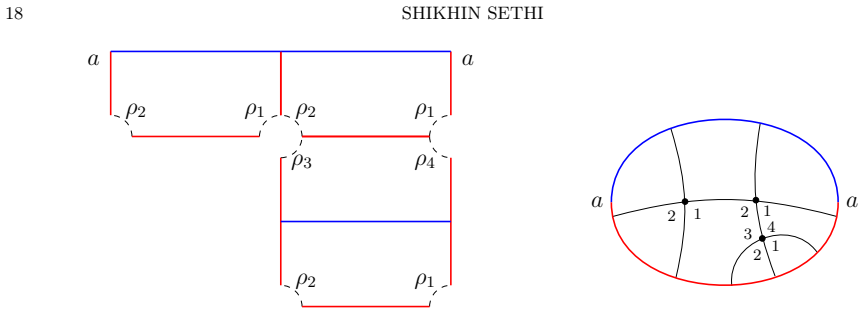
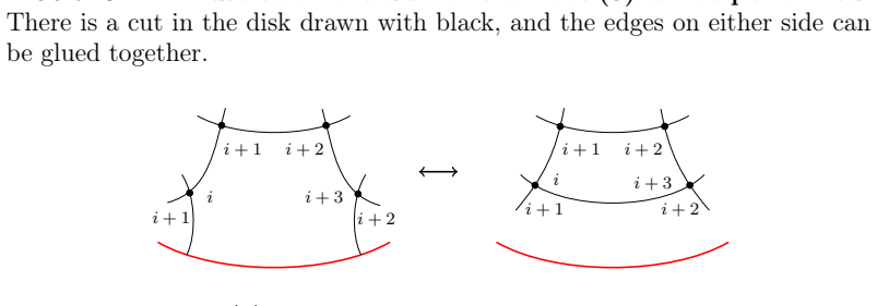
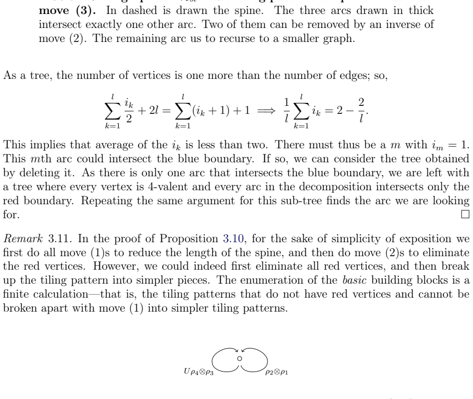
The central object is the module tiling pattern: a planar graph embedded in the disk, with blue boundary mapping to the $\beta$-circle and red boundary to the $\alpha$-arcs, four-valent internal vertices away from the boundary, valid $\mathbb{Z}/4$ labelings around vertices, and weight equal to the number of internal faces, called short cycles. The three moves are (1) gluing two disks along a shared $\alpha$-arc when the adjacent Reeb chord product is non-zero, (2) inserting a copy of the torus by adding a red vertex, and (3) gluing the two sides of a length-four Reeb chord to create an internal face. These moves generate every contributing immersion from the building blocks, and they carry the $A_\infty$ proof: each non-zero term in an $A_\infty$ relation is paired with the tiling-pattern transformation inverse to the corresponding move. The algebraic bridge to type D modules is the weighted module diagonal primitive, which turns the type A counts into a type D structure by box tensor product with the dualizing bimodule $\mathrm{CFDD}^-(I)$.

What would settle it

Enumerate all index-one module tiling patterns for $C_3$ or $C_4$ by an independent search of the dual graph; if any pattern is not generated by the three moves from the Figure 25 building blocks, or if a generated operation violates an $A_\infty$ relation, the construction is incomplete.

Watch

Extended reading notes

Core claim

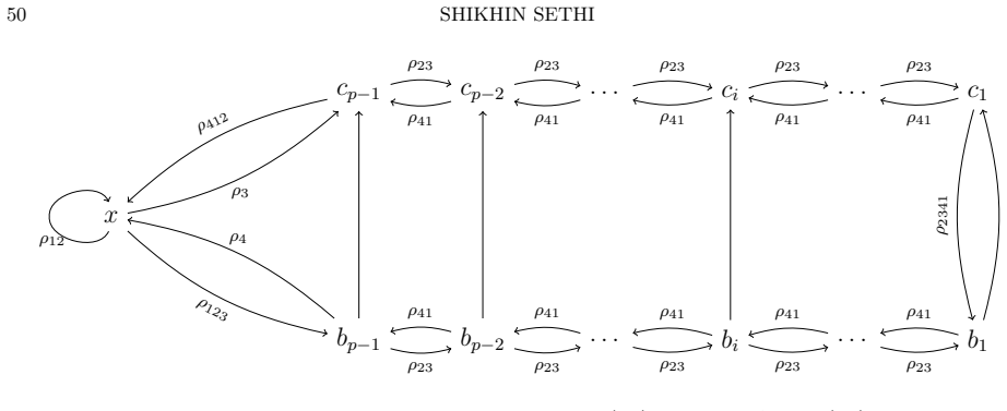
For the bordered Heegaard diagram $C_p$ of the $(p,1)$-cable, the paper defines a weighted $A_\infty$-module $\mathrm{CF} A^-(C_p)$ over the enriched torus algebra $A^{U,V}_-$ with generator $x$ and generators $b_1,\dots,b_{p-1}$, $c_1,\dots,c_{p-1}$. A module operation $m^w_{1+n}(x,a_1,\dots,a_n)$ is the mod-2 sum of all module tiling patterns of weight $w$ and chord sequence $a_1\otimes\cdots\otimes a_n$ obtained from the building blocks of Figure 25 by the three moves of Section 3.1.2; the weight counts short cycles, the chord sequence records the Reeb chords read along the red boundary, and the output carries powers of $U$ and $V$ tracking the two basepoints. The paper proves the $A_\infty$ structure relations by pairing the non-zero terms of each relation and cancelling them over $\mathbb{F}_2$, with each cancellation corresponding to one of the moves or to splitting a tiling pattern along the blue or red boundary. The uniqueness theorem states that if $M$ is any graded weighted $A_\infty$-module whose $V=0$ reduction is the known hat module of the $(p,1)$-cable, then the box tensor product $M_{U,V=1}\boxtimes \mathrm{CFDD}^-(I)$ is isomorphic to $\mathrm{CF} A^-_{U,V=1}(C_p)\boxtimes \mathrm{CFDD}^-(I)$, so the associated type D module $\mathrm{CFD}^-(C_p)$ is forced.

Load-bearing premise

The load-bearing premise is that the building blocks of Figure 25 generate every contributing immersed disk for the $(p,1)$-cable; the paper asserts the enumeration is a finite calculation that repeats the $C_2$ analysis 'word for word,' but does not draw the general patterns.

Editorial extensions

If this is right

For any companion knot $K$, the unspecialized knot Floer complex of its $(p,1)$-cable can in principle be obtained by tensoring $\mathrm{CF} A^-(C_p)$ with the type D module of $K$, replacing analytic curve counts by finite graph counts.
The uniqueness theorem means that the minus-flavor type D module is independent of how one extends the hat module, so computations starting from known hat data give the same answer.
Because the $A_\infty$ relations are established by explicit cancellations, the construction is suitable for computer verification and automated enumeration of operations.
The same schema is expected to extend to other $(1,1)$-pattern knots, so the planar-graph calculus may apply to a whole family of satellite operators beyond the $(p,1)$-cables.

Reading between the lines

Editorial extensions of the paper, not claims the author makes directly.

A direct way to test the completeness of the building-block enumeration is to implement the three moves and enumerate all tiling patterns for a small fixed $p$; any index-one disk not generated would expose a missing block.
If the uniqueness theorem generalizes, it suggests that for many bordered diagrams the minus invariant carries no data beyond the hat module together with the gradings and $A_\infty$ relations, a substantial simplification for computations.
The same tiling formalism could be iterated: after computing $\mathrm{CF}A^-(C_p)$, composing it with another pattern's module would give a combinatorial calculus for iterated satellite operations.
The strongest end-to-end test is to compute the full knot Floer complex of a family of $(p,1)$-cables once the pairing theorem appears and compare with existing immersed-curve computations on cases not checked in the paper.

Share X Bluesky LinkedIn Reddit HN

Editorial analysis

A structured set of objections, weighed in public.

Desk editor's note, referee report, and a circularity audit.

Desk Editor's Note

read the letter

Here's my take on Sethi's arXiv:2506.04222. The headline: it gives the first explicit combinatorial models for the minus-flavor bordered Heegaard Floer modules of (p,1)-cables, and the construction is mostly convincing. But the completeness of the basic building-blocks enumeration for general p is asserted with "word for word" and "finite calculation" rather than demonstrated, and that's the one thing I'd want to see before trusting the main theorem.

What's actually new: the weighted A∞-modules CF A^-(C_p), with operations counting planar graph tilings; the combinatorial verification of the A∞ relations via the three moves; the boundedness (filtered bonsai) argument; and the uniqueness theorem saying any graded weighted extension of the hat module has the same associated type D module. Petkova computed only the hat flavor, and LOT's minus theory didn't have explicit modules for these patterns. So this is a genuine step forward. The checks against Petkova's hat computation and the Hom-Kang-Park-Stoffregen UV=0 tensor product are good evidence that the construction is on target.

Where are the soft spots? First, the completeness of the module tiling pattern enumeration for general p. Proposition 3.16 says the analysis repeats "word for word" from C_2, and Remark 3.11 calls it a finite calculation, but the building blocks themselves are not drawn for general p. The C_2 proof already leans on a spine-decomposition argument that the author admits "can get hairy." If a building block were missing, the operations would differ from the true CF A^-(C_p), the A∞ cancellations could break, and the uniqueness theorem wouldn't help identify the constructed module. So this is a real gap, though probably fillable. A referee should ask for the explicit enumeration or a cleaner proof.

Second, the pairing theorem [LOTon] is in preparation. The algebraic results stand without it, but the claim that these are the bordered minus invariants in Section 5 depends on it. The paper is honest about this, but it does limit how much we can extract right now.

Third, a minor point: the analytic-to-combinatorial correspondence (Propositions 3.2 and 3.9) is inherited by citation. That's standard, and not a problem here.

The gradings and the boundedness argument look solid; the case analysis for the A∞ relations is systematic and I didn't find internal contradictions. The paper is written for specialists in bordered Floer and knot Floer homology. It deserves a serious referee. I'd recommend engaging with it, with the expectation of a revision that spells out the general-p enumeration.

Referee Report

4 major / 5 minor

Summary. The paper constructs weighted A-infinity modules CF A^-(C_p) for the (p,1)-cable pattern over the bordered minus torus algebra, with operations defined by counting decorated planar graphs (module tiling patterns) generated from the building blocks of Figure 25 by the three moves of Section 3.1.2. The main theorems claim that these modules satisfy the A-infinity relations (Theorem 3.17), are filtered bonsai (Proposition 4.5), and that any graded weighted extension of the hat module has the same associated type D module as the constructed one (Theorem 4.16). Section 5 computes a sample tensor product with a 1-by-1 rectangle type D structure and reports agreement with the UV=0 computation of Hom, Kang, Park, and Stoffregen.

Significance. If the construction is correct, this is a substantial step toward combinatorial, computable minus-flavor bordered invariants for satellite patterns, extending Petkova's hat-level computation and providing a route to unspecialized knot Floer complexes of satellite knots. The paper has real strengths: the constructions are explicit, the A-infinity relations are addressed by a systematic and detailed case-by-case pairing scheme (T-1 through T-10, TC-1 through TC-10, TC'-3), and the resulting modules are checked against independent external computations. The uniqueness theorem for associated type D modules is a valuable structural result. However, the central claim for general p rests on an enumeration whose completeness is asserted rather than proved, and the satellite-computation interpretation depends on a pairing theorem that is cited to unpublished work.

major comments (4)

[§3.2.2, Proposition 3.16 and Remark 3.11] The completeness of the building-block enumeration for general p is load-bearing but is not proved. The proof of Proposition 3.16 says the analysis of Proposition 3.13 and Proposition 3.14 can be repeated 'word for word,' and Remark 3.11 calls the enumeration of basic building blocks 'a finite calculation,' yet the tiling patterns for general p are not drawn and the C_2 proof already relies on a spine-decomposition argument whose general form is only sketched. If a building block were missing, the operations defined by counting module tiling patterns would differ from the true CF A^-(C_p), and the cancellation proof of Theorem 3.17, especially the TC'-3 analysis, would not be exhaustive. Please supply either a complete proof of Proposition 3.16 or a verifiable finite enumeration (table, algorithm, or machine-checked code) for all p.
[§2.8, Theorem 2.21 and §5] The interpretation of the tensor products as knot Floer complexes of satellites depends on the minus-flavor pairing theorem, which is cited to [LOT23, Theorem 1.36] and to the unpublished item [LOTon]. The algebraic results of Sections 3 and 4 stand independently, but the abstract's claim that the modules 'provide a recipe to compute knot invariants associated to satellite knots' is conditional on this forthcoming pairing theorem. The paper should either prove the needed pairing statement, restrict the claim explicitly as conditional, or replace the citation once a published version is available.
[§4.3, Theorem 4.16] Theorem 4.16 proves that any graded weighted extension of the hat module has the same associated type D module as the constructed module; it does not prove that the constructed module is homotopy equivalent to the analytically defined bordered minus invariant CF A^-(C_p). The paper itself notes that quasi-invertibility of CFDD^-(I) is expected but not established. Without that step, the uniqueness result does not fully justify the abstract's wording that the paper 'combinatorially constructs' the actual weighted A-infinity modules. Please either prove the needed quasi-invertibility or state the result in the weaker, precisely proved form.
[§4.2, Proposition 4.5] The filtered-bonsai proof relies on the assertion that operations with total U plus V power zero form no directed cycles. This assertion is stated without proof, after only a brief description of the zero-total-power subgraph of Figure 25 and its closure under move (1). Because filtered bonsai is needed for the tensor products to be well-defined, this point is load-bearing for Section 5. Please provide an explicit argument, for example a monotone grading quantity that prevents directed cycles, or a direct analysis of all possible compositions in Figure 25.

minor comments (5)

[§3.2.2, Proposition 3.16] The phrase 'We can repeat, word for word, the analysis' is too informal for the proof of a proposition that is central to the paper; even if the full enumeration is deferred, the proof should indicate which specific arguments and definitions from Propositions 3.13 and 3.14 carry over and what changes for general p.
[Theorem 3.15, TC-3 example] There is an unbalanced parenthesis in the displayed cancellation: 'm0_5((m0_6(x, ρ3, ρ234, ρ3, ρ2, ρ12), ρ12, ρ1, ρ4, ρ34)' contains an extra opening parenthesis and is missing a closing parenthesis.
[Theorem 3.17, TC'-3] In the sentence describing cancellation against a curvature term, 'mw−1 2+n (x, a1, . . . , an), µ1 0)' has a misplaced closing parenthesis; it should read 'mw−1 2+n (x, a1, . . . , an, µ1 0)'.
[Figure 25] Figure 25 is very dense and the labels such as U^{p-2}, U^i, U^{p-1}, and the repeated ρ2⊗ρ1 / ρ4⊗ρ3 blocks are hard to read in print; a table listing each building-block operation along with its input chord sequence, output generator, and U,V powers would substantially improve verifiability.
[§4.2, Proposition 4.5] The symbol n is used both for the number of inputs in m^w_{1+n} and for the fixed total U plus V power in the statement 'where the total power k + l = n'; renaming one of these quantities would avoid confusion.

Circularity Check

0 steps flagged · score 0.0 of 10

No significant circularity: the construction is self-contained apart from explicitly flagged external dependencies.

full rationale

The paper's derivation chain is not circular. The module operations on CFA^-(C_p) are defined by counting module tiling patterns associated to immersed disks, and the three moves of Section 3.1.2 are geometric operations whose index behavior is proved from the embedded index formula (Proposition 3.8). The completeness propositions (3.10, 3.14, 3.16) are assertions that all operations arise from the displayed building blocks; they do not define the operations in terms of the conclusion. The A-infinity relation proofs (Theorems 3.12, 3.15, 3.17) pair nonzero terms via explicit inverse geometric operations, using the published algebra structure of A^- from [LOT21] as an external input; they do not assume the A-infinity relations. The uniqueness theorem (Theorem 4.16) is a new statement comparing arbitrary graded weighted extensions and does not presuppose the constructed module's identification. The sample tensor product in Section 5 is checked against the independent computation of Hom, Kang, Park, and Stoffregen, and the hat-flavor agreement with Petkova is noted as external verification. The paper explicitly flags the two genuine gaps: the pairing theorem is cited to the in-preparation work [LOTon] (Section 2.8), and the general-p enumeration of basic building blocks is deferred with 'We can repeat, word for word' and 'a finite calculation' (Section 3.2.2, Remark 3.11). These are missing-support or omitted-proof concerns, not circularity. No load-bearing step reduces by construction to its own inputs.

Assumptions & free parameters 0 free parameters · 8 assumptions · 0 invented entities

The paper contributes no fitted constants. It rests on the published minus-flavor framework of Lipshitz, Ozsváth, and Thurston, on classical pseudo-holomorphic counting results, and on two internal assertions (building-block completeness and the acyclicity claim) that would benefit from explicit verification.

assumptions (8)

domain assumption The torus algebra A^- is a weighted (curved) A∞-algebra with operations counting tiling patterns, with curvature µ1_0 = ρ1234 + ρ2341 + ρ3412 + ρ4123.
Section 2.2 cites [LOT21] for this structure; every module operation and every A∞-relation verification relies on these algebra operations and their relations.
standard math Embedded index formula (Proposition 2.17) and its consequences (Lemma 2.19, Proposition 2.20), used in Proposition 3.8 to show the three moves preserve index 1.
Quoted from [LOT21] and [LOT23]; the combinatorial description needs the identification of index-1 moduli spaces with the described planar graphs.
domain assumption An immersed disk for the genus-one bordered diagram with acute corners at the marked intersections has exactly one pseudo-holomorphic representative modulo 2 (Proposition 3.2), and disks with obtuse corners have index greater than 1 (Proposition 3.9).
Proposition 3.2 is cited to [Han14] and Proposition 3.9 to [Pet13; Hom13]; these identify the planar graph counts with the analytic definition of CF A^-.
domain assumption The pairing theorem for the minus flavor, CF^-(Y2 ∪ Y1) ≃ CF A^-(Y2) ⊠ CFD^-(Y1), holds (Theorem 2.21).
Cited to [LOT23, Theorem 1.36] and [LOTon], which the author states is 'In preparation'; it is needed to interpret the sample tensor product in Section 5 as knot Floer data.
domain assumption A compatible weighted algebra diagonal and module diagonal primitive from [LOT20] exist, and the box tensor products are defined through the fixed choices; independence of choices is cited to [LOT23, Proposition 7.7].
Used in Sections 2.4 and 4.3 to define CFDD^-(I), CFD^-, and the tensor products M ⊠ CFDD^-(I).
domain assumption The type DD dualizing bimodule CFDD^-(I) has the differential of Equation (4.6), inherited from [LOT23].
This fixed bimodule is the bridge between type A and type D modules in the uniqueness theorem.
ad hoc to paper The operations generated by Figure 25 with total U plus V power zero form no directed cycles (used to prove filtered-bonsai in Proposition 4.5).
This is asserted in the proof of Proposition 4.5 rather than demonstrated; if false, the boundedness argument fails.
ad hoc to paper The completeness of the building-block enumeration for C_p (Proposition 3.16).
The completeness of the descriptions of all operations is asserted by repeating the C_2 argument; the finite calculation is not exhibited.

how reviews work

0 comments

Cite this review

Pith. "Pith review of Bordered Heegaard Floer modules for satellite operations using planar graphs." pith.science (2026). https://pith.science/paper/Z5DZGCPV

@misc{pith2026250604222,
  author       = {Pith},
  title        = {Pith review of: Bordered Heegaard Floer modules for satellite operations using planar graphs},
  year         = {2026},
  howpublished = {\url{https://pith.science/paper/Z5DZGCPV}},
  note         = {Machine review of arXiv:2506.04222}
}

abstract

Lipshitz, Ozsv\'ath, and Thurston extend the theory of bordered Heegaard Floer homology to compute $\mathbf{CF}^-$. Like with the hat theory, their minus invariants provide a recipe to compute knot invariants associated to satellite knots. We combinatorially construct the weighted $A_\infty$-modules associated to the $(p, 1)$-cable. The operations on these modules count certain classes of inductively constructed decorated planar graphs. This description of the weighted $A_\infty$-modules provides a combinatorial proof of the $A_\infty$ structure relations for the modules. We further prove a uniqueness property for the modules we construct: any weighted extensions of the unweighted $U = 0$ modules have isomorphic associated type D modules.

Figures

Figures reproduced from arXiv: 2506.04222 by the authors.

**Figure 1.** Examples of tiling patterns. The root on the boundary is marked with the black dot. On the left is a centered tiling pattern. On the right, a left-extended one. • If e : v1 → v2 is an edge oriented such that a face f is to the right of e, then Λv1 (f) + 1 ≡ Λv2 (f) mod 4. is maintained. To each tiling pattern Γ, we associate a weight w ∈ Z≥0, a chord sequence a1 ⊗ · · · ⊗ an where each ai ∈ A−, and an output o ∈ A−.… view at source ↗

**Figure 2.** A bordered Heegaard diagrams Hst for the 0-framed solid torus. The intersection of the α-arc and the β-circle is a. There is a marked point z near the boundary with Reeb chord ρ4. 2.8. Pairing theorems. The dream of bordered Heegaard Floer theory is to recover the Heegaard Floer invariant of a manifold by pairing the type A and type D invariants of the pieces. At the time of writing this paper, pairing theorems for … view at source ↗

**Figure 3.** The dual graph for the 0-framed solid torus. The bordered Heegaard diagrams is given by the thick red arcs and the thick blue curve. The black nodes are the vertices in Γ(Hst). The edges in Γ β (Hst) are dotted purple, and the remaining edges in Γ(Hst) are grey. the structure relations on CFA− , as the operations on the algebra A− are constructed with similar classes of planar graphs. Given a bordered Heegaard diagr… view at source ↗

Figures from the paper (29 more)

**Figure 4.** Figure 4: An immersed disk and its corresponding module tiling pattern. A module tiling pattern consists of such a planar graph Γ(u) along with additional data. Along the intersections of the red and the blue boundaries of the disk, we mark x and y for u an immersion from x to y…

**Figure 5.** Figure 5: An illustration of disks where move (1) can be performed. The two disks can be glued along the shaded edge. This results in the disk from [PITH_FULL_IMAGE:figures/full_fig_p020_5.png]

**Figure 6.** Figure 6: Move (1) on module tiling patterns. The labeling near the vertex is forced by the condition that ana ′ 1 ̸= 0. The move identifies the two edges to the red boundary on the left. i i + 3 i i + 3 i + 1 i i + 3 i + 2 [PITH_FULL_IMAGE:figures/full_fig_p020_6.png]

**Figure 7.** Figure 7: Move (2) on module tiling patterns. The move adds a new vertex with labelings as illustrated. identified with the first edge to the red boundary of the first pattern. This is illustrated in [PITH_FULL_IMAGE:figures/full_fig_p020_7.png]

**Figure 8.** Figure 8: An illustration of a disk where move (3) can be performed. There is a cut in the disk drawn with black, and the edges on either side can be glued together. i + 1 i + 2 i i + 3 i + 1 i + 2 i i + 3 i + 1 i + 2 i + 1 i + 2 [PITH_FULL_IMAGE:figures/full_fig_p021_8.png]

**Figure 9.** Figure 9: Move (3) on module tiling patterns. The move creates a new internal face, and the labelings remain unchanged. The labelings around the newly formed edge remain consistent by virtue of the labeling conventions around vertices, as depicted in the figure. Move (3): Consid…

**Figure 10.** Figure 10: An illustration of a disk with an obtuse angle at the α-arc and β-circle boundary. There is a cut in the disk indicated by the black line, and a branch point at the end of the cut. When the boundary branch point goes out to the α-arc, the disk decomposes into two disk…

**Figure 11.** Figure 11: The building blocks for operations for the 0-framed solid torus. structure of this are depicted in [PITH_FULL_IMAGE:figures/full_fig_p024_11.png]

**Figure 12.** Figure 12: The structure of a module tiling pattern for Hst near the blue boundary. The horizontal arc is the spine. The graph Γ(u) is connected and planar. Away from the blue boundary, ever vertex of Γ(u) is 4-valent, and every internal face is bound by four edges. This is enti…

**Figure 13.** Figure 13: A graph for Hst illustrating possible simplifications with move (3). In dashed is drawn the spine. The three arcs drawn in thick intersect exactly one other arc. Two of them can be removed by an inverse of move (2). The remaining arc us to recurse to a smaller graph. …

**Figure 14.** Figure 14: A representation of the type A module CFA− (Hst). The type A module CFA− (Hst) can be represented by the graph in [PITH_FULL_IMAGE:figures/full_fig_p025_14.png]

**Figure 15.** Figure 15: The term cancellations in (T-2) in Theorem 3.12. On the left, the first module tiling pattern is drawn on the bottom, and the second on the top. The tiling pattern for the centered algebra operation is on the right. For example, in the weight 0 A∞ relation with inputs…

**Figure 16.** Figure 16: The term cancellations in (T-3) in Theorem 3.12. On the left, the first module operation is drawn on the bottom, and the second on the top. The labels are arbitrarily chosen. Top: pushing out the edge e to the red boundary punctures an internal face, producing a modul…

**Figure 17.** Figure 17: The term cancellations in (T-4) in Theorem 3.12. The labels are arbitrarily chosen. Left: a module tiling pattern with a chord factorized as the product of aj and aj+1. Right: pushing out the edge corresponding to the factorization to the red boundary produces a comp…

**Figure 18.** Figure 18: An immersed disk corresponding to the term cancellation in (T-7) in Theorem 3.12. There is a cut in the disk along the shaded edge, such that the first Reeb chord is ρ4123. Gluing this and cutting along the black line decomposes the disk into two disks, the module ti…

**Figure 19.** Figure 19: A bordered Heegaard diagram C2 for the (2, 1)-cable, and its dual graph. We can now breathe. We have considered the contribution to the A∞ relations of every weighted tree with two internal vertices, and shown how to pair these contributions up so they cancel. This ve…

**Figure 20.** Figure 20: The building blocks for operations for the (2, 1)-cable. Proposition 3.14. Any operation on the type A module CFA− (C2) can be obtained as the operation associated to a module tiling pattern constructed by starting with the building blocks in [PITH_FULL_IMAGE:figures…

**Figure 21.** Figure 21: A representation of the type A module CFA− (C2). The type A module CFA− (C2) can be represented by the graph in [PITH_FULL_IMAGE:figures/full_fig_p035_21.png]

**Figure 22.** Figure 22: The term cancellations in (TC-2) of Theorem 3.15. On the left, the first module operation is drawn on the bottom, and the second on the top. The lengths of the blue boundaries match, and the two tiling patterns glue together to give a centered algebra operation on the…

**Figure 23.** Figure 23: The term cancellations in (TC-3) of Theorem 3.15. On the left, the first module operation is drawn on the bottom, and the second on the top. The vertex e ∩ e ′ is 2-valent, and pushing out the edge e to the red boundary produces a composite pattern Γ1 # Γ2 where Γ1 an…

**Figure 24.** Figure 24: A bordered Heegaard diagram Cp for the (p, 1)-cable. (TC-7) Consider terms of the form mw−1 2+n (x, µ1 0 , a1, . . . , an) or mw−1 2+n (x, a1, . . . , an, µ1 0 ). These terms were cancelled against in (TC-3). The inverse admits a clean description in terms of the imme…

**Figure 25.** Figure 25: A representation of the type A module CFA− (Cp). Proposition 3.16. Any operation on the type A module CFA− (Cp) can be obtained as the operation constructed by starting with the operations recorded in the graph in [PITH_FULL_IMAGE:figures/full_fig_p040_25.png]

**Figure 26.** Figure 26: A module tiling pattern for C4. The operation is m0 1 (b3) = U 3 c3. The corresponding immersed disk is drawn on the left in solid purple in [PITH_FULL_IMAGE:figures/full_fig_p041_26.png]

**Figure 27.** Figure 27: Immersed disks representing a cancellation in (TC′ -3) of Theorem 3.17. In solid purple is an immersed disk for Γ1 and in hatched green is an immersed disk for Γ2, in the notation of (TC′ -3). The composition of operations on left cancels against the composition of op…

**Figure 28.** Figure 28: Immersed disks representing cancellations for the Whitehead double. The two illustrations on the left cancel against each other, and are analogous to the cancellation of [PITH_FULL_IMAGE:figures/full_fig_p043_28.png]

**Figure 29.** Figure 29: The tensor product CFD − (Hst) = CFA− U=1(Hst) ⊠AU=1 − CFDD − (I). Proof. We abbreviate the generator x⊗(ι1⊗ι1) of the tensor product CFD − (Hst) as x. Both terms in δ 1 (x) = ρ41 ⊗x+ρ23 ⊗x follow from the chosen weighted module diagonal primitive p 3,0 . On the seque…

**Figure 30.** Figure 30: The tensor product CFD − (Cp) = CFA− U,V =1(Cp) ⊠AU=1 − CFDD − (I). ρ2341 ⊗ c1 in the structure relations that arise from µ 1 0 ⊗ b1 and µ 1 0 ⊗ c1, and the only term permissible with the gradings that can cancel them is δ 1 (c1) having a term ρ2341 ⊗ b1. We recap our…

**Figure 31.** Figure 31: A 1 × 1 rectangle and the associated weighted type D module. On the right is illustrated the relative spinc -gradings. The only non-zero term that remains is the composition me 0 3 (m0 3 (ebp−i , ρ2, ρ1), ρ4, ρ3), where we know m0 3 (ebp−i , ρ2, ρ1) = Uebp−(i+1). To c…

**Figure 32.** Figure 32: Summands of the tensor product of CFA− (Cp) with the type D structure of a 1 × 1 rectangle as in [PITH_FULL_IMAGE:figures/full_fig_p052_32.png]

Discussion (0). Sign in to comment.

Reference graph

Works this paper leans on

5 extracted references · 1 canonical work pages

[1]

Satellite knots and immersed Hee- gaard Floer homology

[CH23] Wenzhao Chen and Jonathan Hanselman. “Satellite knots and immersed Hee- gaard Floer homology” (2023). eprint:arXiv:2309.12297. [CZZ24] Daren Chen, Ian Zemke, and Hugo Zhou. “L-space satellite operators and knot Floer homology” (2024). eprint:arXiv:2412.05755. [GMM05] Hiroshi Goda, Hiroshi Matsuda, and Takayuki Morifuji. “Knot Floer Homology of (1, ...

arXiv 2023
[400]

Holomorphic triangles and invariants for smooth four-manifolds

eprint: arXiv:math/0110169. [OS08] Peter Ozsváth and Zoltán Szabó. “Knot Floer homology and integer surgeries”. Algebraic & Geometric Topology8.1 (Feb. 2008), pp. 101–153. [OS22] Peter S. Ozsváth and Zoltán Szabó. “The pong algebra” (2022). eprint: arXiv: 2212.11885. [OS23] Peter S. Ozsváth and Zoltán Szabó. “Planar graphs deformations of bordered knot al...

work page Pith review arXiv 2022
[2003]

An algorithm for computing some Heegaard Floer homologies

eprint:arXiv:math/0306378. [SW10] Sucharit Sarkar and Jiajun Wang. “An algorithm for computing some Heegaard Floer homologies”. Annals of Mathematics 171.2 (Mar. 2010), pp. 1213–1236. eprint: arXiv:math/0607777. [Zem21] Ian Zemke. “Bordered manifolds with torus boundary and the link surgery for- mula” (2021). eprint:arXiv:2109.11520

arXiv 2021
[2006]

Bimodules in bor- dered Heegaard Floer homology

[LOT15] Robert Lipshitz, Peter S. Ozsváth, and Dylan P. Thurston. “Bimodules in bor- dered Heegaard Floer homology”.Geom. Topol.19.2 (2015), pp. 525–724. eprint: arXiv:1003.0598. [LOT18] Robert Lipshitz, Peter S. Ozsváth, and Dylan P. Thurston. “Bordered Heegaard Floer homology”.Mem. Amer. Math. Soc.254.1216 (2018), pp. viii+279. eprint: arXiv:0810.0687. ...

arXiv 2015
[2014]

Knot Floer homology as immersed curves

[Han23] Jonathan Hanselman. “Knot Floer homology as immersed curves” (2023). eprint: arXiv:2305.16271. [Hed05] MatthewHedden.“OnknotFloerhomologyandcabling”. Algebraic & Geometric Topology 5.3 (Sept. 2005), pp. 1197–1222. eprint:arXiv:math/0406402. [Hom+22] Jennifer Hom et al. “Linear independence of rationally slice knots”.Geometry & Topology 26.7 (Dec. ...

arXiv 2023

Pith tools

Reviewed August 7, 2026 · model on record in the stance chip above.

[1] [1]

Satellite knots and immersed Hee- gaard Floer homology

[CH23] Wenzhao Chen and Jonathan Hanselman. “Satellite knots and immersed Hee- gaard Floer homology” (2023). eprint:arXiv:2309.12297. [CZZ24] Daren Chen, Ian Zemke, and Hugo Zhou. “L-space satellite operators and knot Floer homology” (2024). eprint:arXiv:2412.05755. [GMM05] Hiroshi Goda, Hiroshi Matsuda, and Takayuki Morifuji. “Knot Floer Homology of (1, ...

arXiv 2023

[2] [400]

Holomorphic triangles and invariants for smooth four-manifolds

eprint: arXiv:math/0110169. [OS08] Peter Ozsváth and Zoltán Szabó. “Knot Floer homology and integer surgeries”. Algebraic & Geometric Topology8.1 (Feb. 2008), pp. 101–153. [OS22] Peter S. Ozsváth and Zoltán Szabó. “The pong algebra” (2022). eprint: arXiv: 2212.11885. [OS23] Peter S. Ozsváth and Zoltán Szabó. “Planar graphs deformations of bordered knot al...

work page Pith review arXiv 2022

[3] [2003]

An algorithm for computing some Heegaard Floer homologies

eprint:arXiv:math/0306378. [SW10] Sucharit Sarkar and Jiajun Wang. “An algorithm for computing some Heegaard Floer homologies”. Annals of Mathematics 171.2 (Mar. 2010), pp. 1213–1236. eprint: arXiv:math/0607777. [Zem21] Ian Zemke. “Bordered manifolds with torus boundary and the link surgery for- mula” (2021). eprint:arXiv:2109.11520

arXiv 2021

[4] [2006]

Bimodules in bor- dered Heegaard Floer homology

[LOT15] Robert Lipshitz, Peter S. Ozsváth, and Dylan P. Thurston. “Bimodules in bor- dered Heegaard Floer homology”.Geom. Topol.19.2 (2015), pp. 525–724. eprint: arXiv:1003.0598. [LOT18] Robert Lipshitz, Peter S. Ozsváth, and Dylan P. Thurston. “Bordered Heegaard Floer homology”.Mem. Amer. Math. Soc.254.1216 (2018), pp. viii+279. eprint: arXiv:0810.0687. ...

arXiv 2015

[5] [2014]

Knot Floer homology as immersed curves

[Han23] Jonathan Hanselman. “Knot Floer homology as immersed curves” (2023). eprint: arXiv:2305.16271. [Hed05] MatthewHedden.“OnknotFloerhomologyandcabling”. Algebraic & Geometric Topology 5.3 (Sept. 2005), pp. 1197–1222. eprint:arXiv:math/0406402. [Hom+22] Jennifer Hom et al. “Linear independence of rationally slice knots”.Geometry & Topology 26.7 (Dec. ...

arXiv 2023