REVIEW 3 major objections 5 minor 78 references
Estimating Bolometric Luminosities of Type 1 Quasars with Self-Organizing Maps
T0 review · 3 major / 5 minor · reviewed 2026-08-07 · deepseek-v4-flash
Pith's one-line read A self-organizing map trained on 11 photometric bands estimates bolometric luminosities of type 1 quasars with about 4.9% scatter, roughly four times better than single-band bolometric corrections.
desk verdict Useful methods paper with code and catalog, and the headline 4.9% scatter should be read as internal precision, not demonstrated absolute accuracy. read the letter →
The pith
A machine-rendered reading of the paper's core claim, the machinery that carries it, and where it could break.
The reading
What carries the argument
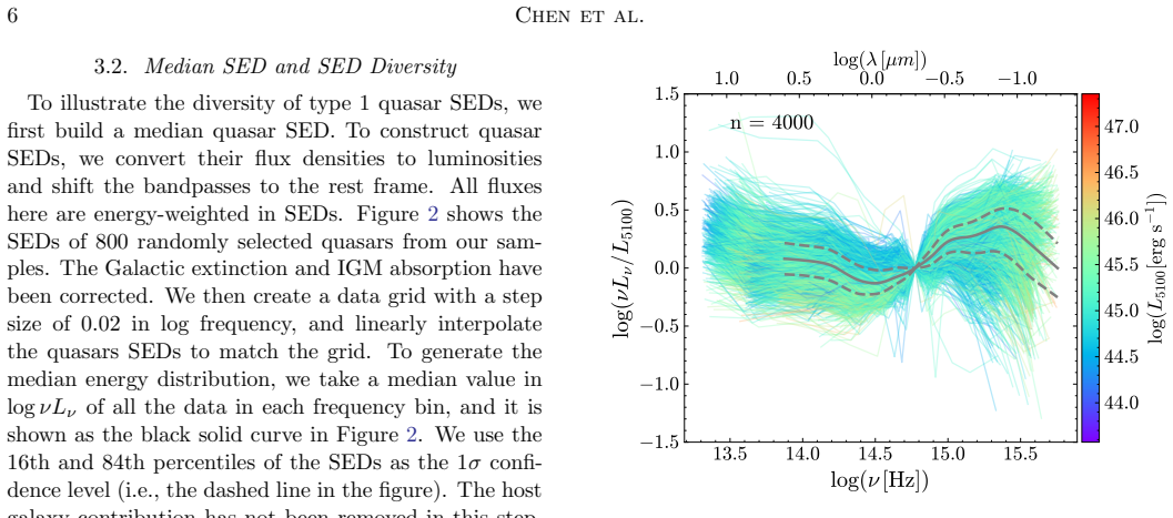
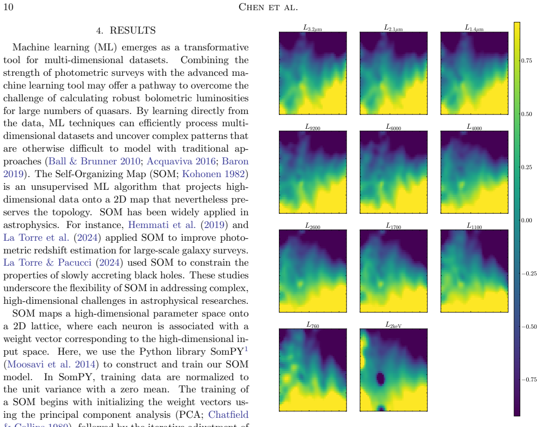
The central object is the self-organizing map (SOM), an unsupervised neural network that projects the 11-dimensional space of observed rest-frame monochromatic luminosities onto a 45$\times$45 grid of cells while preserving topological order. After training on 80% of the fiducial sample, each cell contains quasars with similar SEDs, and the median and dispersion of the true $\log L_{\rm bol}$ within that cell are assigned to any new quasar whose best-matching cell is found. Missing bands, notably W3 and W4, are filled with k-nearest-neighbor imputation before projection, which lets the same trained map handle quasars with limited photometry. The map's topology-based averaging is what converts multi-band SED similarity into a luminosity estimate.
What would settle it
Take a subsample of quasars with actual X-ray detections and individually decomposed host galaxies, compute $L_{\rm bol}$ by integrating the observed SEDs from the far-IR to hard X-rays, and compare with SOM estimates from the released code; if the scatter is substantially larger than $\sigma_f\approx 5\%$ or shows a luminosity-dependent offset, the small scatter is an artifact of training and testing on the same corrected photometry.
Extended reading notes
Core claim
The paper's central claim is that a 45$\times$45 self-organizing map trained on 11 rest-frame monochromatic luminosities reproduces the bolometric luminosities of type 1 quasars with fractional residual scatter $\sigma_f \approx 4.9\%$, compared with 18$-$29% for single-band bolometric corrections and 13.6% for three-band multiple linear regression. The map is trained on SEDs constructed from multi-band photometry after corrections for Galactic extinction, IGM absorption, host-galaxy contamination, and emission lines, and each cell's median $\log L_{\rm bol}$ becomes the estimator for any quasar mapped to that cell. The authors apply the trained model to 633,373 SDSS DR16Q quasars, release the code and the resulting catalog, and recalculate bolometric corrections at 1450, 3000, 5100, and 10,000 \AA{} rest-frame wavelengths together with updated multi-linear regression relations.
Load-bearing premise
The load-bearing premise is that the 'true' luminosities used to train and test the map are accurate, since they come from integrating the same corrected photometry that feeds the map; any bias in the host-galaxy, intergalactic-medium, or predicted X-ray corrections would move targets and estimates together, and the paper itself notes that only interpolation error is included in its uncertainties, so the 4.9% scatter does not bound the absolute error.
Editorial extensions
If this is right
- For the 633,373 DR16Q quasars with released estimates, bolometric luminosities now come with documented per-object systematic uncertainties instead of a single assumed bolometric correction.
- Recalibrated bolometric corrections at 1450, 3000, and 5100 \AA{} (2.93, 3.72, and 6.43) make the luminosity dependence of the correction explicit, so future work can avoid the bias of a constant bolometric correction.
- Quasars with incomplete photometry remain usable: KNN-imputed SEDs recover $L_{\rm bol}$ with $\sigma_f$ of roughly 13$-$16% when four to eight bands are available.
- Because the method handles a wide range of luminosity and redshift and needs no low-resolution SED fitting, it can be applied directly to the next generation of wide multi-band quasar samples.
Reading between the lines
- One extension the authors leave implicit is that the same trained map can serve as a general SED classifier, predicting any rest-frame band luminosity or color from partial photometry, not just $L_{\rm bol}$.
- Because 85% of the training targets use X-ray luminosities predicted from the UV relation, the 4.9% figure should be read as precision relative to those corrected targets; an absolute check needs quasars with measured X-ray fluxes and individually decomposed host galaxies.
- The paper's own limited-data tests imply that UV coverage, not IR coverage, controls accuracy: dropping to four NUV-to-optical bands raises $\sigma_f$ to about 14%, so future surveys that add near-UV photometry will benefit most.
Editorial analysis
A structured set of objections, weighed in public.
Referee Report
Summary. This paper proposes a self-organizing map (SOM) method for estimating bolometric luminosities of unobscured type 1 quasars from multi-band photometry. The authors build a fiducial sample of 79,163 SDSS DR16 quasars at 0.5≤z≤2 with GALEX, SDSS, UKIDSS/UHS/VHS, WISE, and X-ray data, correct for Galactic extinction, IGM absorption, host galaxy contamination, and emission lines, integrate the rest-frame SEDs over 4 µm–10 keV to define Lbol, and train a 45×45 SOM on 11 monochromatic luminosities from 3.2 µm to 2 keV. They report a fractional residual dispersion σf≈4.9% against their own Lbol values, substantially smaller than single- or multi-band linear regression and bolometric corrections, and they apply the method to 633,373 DR16Q quasars, releasing code and a catalog.
Significance. If the claimed accuracy were absolute, the method would be a valuable community resource: it is fast, uses SED diversity rather than a single band, includes a held-out test set, checks selection effects, tests limited-data recovery, and ships public code and a large catalog. The comparison with bolometric corrections and linear regressions on the same labels is internally instructive and demonstrates that the SOM recovers the authors' own Lbol definition far better than single-band methods. However, the central claim that the method 'reduces systematical uncertainties' is not yet supported, because the labels are constructed from the same photometry that provides the SOM inputs; the small σf measures self-consistency, not absolute accuracy. The only independent comparison, against Wu & Shen (2022), shows a median offset an order of magnitude larger than the quoted scatter.
major comments (3)
- [§4.3, §4.5, Figs. 10 and 13] The central quantitative claim, σf≈4.9% in §4.3/Figure 10, is a recovery test of the authors' own Lbol definition. The 'true' Lbol is obtained by integrating SEDs built from the same photometric bands that form the 11 SOM inputs, after the same corrections: IGM absorption (§3.1), host galaxy subtraction (§3.3), emission-line corrections (§3.4), interpolation/imputation (§3.5), and the Steffen et al. X-ray relation for 85% of sources (§2.4). Biases in any of these corrections shift labels and features coherently, so the small residual scatter does not bound the absolute error. This is not only a philosophical point: §4.5/Figure 13 reports a 14.8% median offset and 43.6% 1σ scatter against the independent Wu & Shen (2022) estimates, an order of magnitude larger than σf. The authors themselves state in §3.5 that 'the uncertainty of bolometric luminosity is underestimated in this work' and in §5 that systematic uncertainties will be characterized in future work. I therefore request an external validation, e.g., comparison with SED-fitting-based Lbol values (Lusso et al. 2012; Duras et al. 2020) for a matched sample, or a simulation with injected SEDs of known Lbol, together with a propagation of the dominant correction uncertainties (host fraction, IGM transmission, Steffen relation scatter) into the predicted Lbol. Without this, the abstract's claim that the method 'reduces systematical uncertainties' is premature.
- [§4.5, §4.6, Table 5] The application to DR16Q in §4.5 and the code's scaling option in §4.6 extrapolate the SOM beyond its training domain. The fiducial SOM is trained on 0.5≤z≤2 quasars, but the released catalog covers z<5 and includes a scaling parameter for faint (log Lbol < 45.13) and bright (>46.74) ends with no validation shown. The IGM transmission correction is extended to z=5 and to u, g, r bands, which were not part of the §3.1 calculation, and the per-source uncertainties in the catalog do not include extrapolation error. I ask for a validation subset (e.g., z>2 or very luminous quasars with X-ray detections or SED-fitting Lbol) or, alternatively, an explicit statement that the claimed σf≈4.9% and the released uncertainties apply only within the training domain.
- [§3.5, §4.1, §4.4] Section 3.5 states that about 20% of the fiducial SEDs do not reach 4 µm and uses KNNImputer to fill in the missing W3/W4 photometry before computing Lbol; these same imputed values enter both the SOM input features and the target labels. The sentence that conclusions remain 'quantitatively consistent' when excluding these samples is not accompanied by the actual numbers. More importantly, it is unclear whether the KNN imputation is performed before the 80/20 train/test split described in §4.1. If the imputation models are fit on the full sample, test objects can contribute to their own imputation, which would artificially lower the test-set σf. Please clarify the order of operations and, if necessary, rerun the test-set validation with imputation fit only on the training set, reporting the affected values.
minor comments (5)
- [§3.1] The text refers to 'Figure 3.1' for the IGM transmission example, but figures are numbered sequentially elsewhere (Figure 1 is the redshift/L2500 plot in §2). Please renumber or reference the actual figure.
- [Table 5] Table 5 lists the default integration range as 'from 4 µm to 2 keV' and describes 'wave range' as being in Hz, while §3.5 and §5 state the default range is 4 µm–10 keV. Please make the default range and units consistent between the text, table, and code.
- [Appendix A, Table 6] The column numbering in Table 6 repeats '4' twice (X RAY MATCHED and Chandra FLUX) and the subsequent column numbers are shifted; the column headings should be renumbered.
- [§2.1] The flag name 'ERRBITS=0' appears to be a typo; if it refers to UKIDSS/UHS quality flags, please use the actual flag names from those catalogs.
- [§4.3] The σf values quoted in the text for the BC method at 1450, 3000, and 5100 Å are given as 20.3%, 18.0%, and 29.0%, while Table 2 reports 0.203, 0.180, and 0.290 in fractional units; please unify the presentation of these numbers.
Circularity Check
The 4.9% scatter is internally anchored: 'true' Lbol and the SOM inputs derive from the same photometry and the same statistical corrections, so the claimed accuracy does not bound absolute systematic error.
-
self definitional
[Sections 3.5 and 4.1 (Eq. 2; SOM input definition)]
"Bolometric luminosity is the integrated area under the SED curve. Its mathematical definition is as follows, Lbol = Z ∞ 0 Lνdν = Z ∞ −∞ ln(10)νLνd log(ν). ... We use an integration range of 4 µm-10 keV (default range) in this paper. ... In this work, the input parameter space has 11 dimensions representing the rest-frame quasar SEDs (i.e., 11 monochromatic luminosities)."
The 11 input features are monochromatic luminosities drawn from the same rest-frame SED whose integral defines Lbol. The label is not an independent measurement: Lbol is a deterministic functional of the same photometry and the same corrections (IGM transmission, host-galaxy fraction, KNN-imputed W3/W4, and the Steffen et al. L_UV-L_X relation for 85% of quasars). A SOM can therefore recover Lbol with small residuals by learning the quadrature-like mapping from the 11 fluxes to their own integral. Any systematic error in the shared corrections shifts inputs and labels together and is invisible in the residual. The train/test split only verifies interpolation of the authors' own Lbol definition, not agreement with an absolute measurement.
-
other
[Section 2.4 (Steffen et al. relation) combined with Section 3.5 (integration range) and Section 4.1 (2 keV input)]
"For quasars without X-ray detections (85%), we estimate their X-ray flux using the correlation defined by the LUV − LX relation based on the luminosities at 2500 Å and 2 keV. Steffen et al. (2006) used 333 quasars ... log(L2keV) = (0.721±0.011) log(L2500)+(4.531±0.688)."
For 85% of the sample, the 2 keV luminosity is not observed but is predicted from L2500. That same predicted 2 keV flux is both one of the 11 SOM inputs and part of the integrated Lbol (the default range is 4 µm-10 keV). Any error in the Steffen relation is therefore common-mode: it enters the features and the label identically and cannot appear in the quoted σf. The reported scatter tests the internal consistency of the adopted corrections, not the absolute accuracy of the X-ray-inclusive Lbol.
full rationale
The paper does not rely on a load-bearing self-citation chain, and the SOM itself is unsupervised with a held-out test set; there is no uniqueness theorem or ansatz smuggled in via citation. The core circularity is structural: the 'true' Lbol used for training and testing is computed by integrating the very SEDs that provide the 11 input features, after the same statistical corrections are applied to both sides. Hence the headline accuracy (σf ≈ 4.9%) measures how well a smooth function of 11 SED points reproduces the integral of those same SED points, not agreement with an independent bolometric measurement. The external comparison with Wu & Shen (2022) shows a median offset of 14.8% and a 1σ scatter of 43.6%, an order of magnitude larger than the quoted σf, confirming that the claimed precision is internal. The MLR relations are also fit and evaluated on the same sample. The released code and catalog remain useful as a fast, reproducible estimator of the authors' own Lbol definition, but the central claim of reduced systematic uncertainty is not yet supported by an absolute accuracy assessment.
Assumptions & free parameters
free parameters (6)
- Host galaxy fraction at 5100 A (Jalan et al. 2023 relation) =
adopted relation, not refitted; reduces Lbol by about 0.05 dex on average
- IGM transmission model parameters =
b=30 km/s; absorber distribution from Faucher-Giguere (2020); power-law index -0.44
- KNNImputer number of neighbors =
100
- SOM map size and training settings =
45x45 map; sampling rate 90%; quantization error 0.11
- Bolometric integration range =
4 um to 10 keV (default)
- Scaling parameter for faint and bright ends =
option in code; thresholds log(Lbol)<45.13 and >46.74
assumptions (8)
- domain assumption Adopted flat cosmology H0=70 km/s/Mpc, Omega_M=0.3, Omega_Lambda=0.7.
- domain assumption Integration of the SED from 4 um to 10 keV yields the bolometric luminosity; reprocessed IR and coronal X-rays are excluded by default.
- domain assumption Isotropic emission is assumed; optional viewing-angle correction f=0.75 from Nemmen and Brotherton (2010).
- domain assumption Steffen et al. (2006) L_UV-L_X relation applies to the 85% of quasars without X-ray detections.
- domain assumption IGM transmission model with Poisson-distributed HI clouds (Faucher-Giguere 2020) correctly describes average LyC and LyL absorption.
- domain assumption Host galaxy fraction at 5100 A from Jalan et al. (2023) and the spiral template of Assef et al. (2010) describe host contamination for this sample.
- domain assumption Mg II equivalent width relations (based on Wu and Shen 2022 continuum fits) can infer Ly alpha, C IV, H beta, and H alpha line fluxes for the K-correction.
- ad hoc to paper GALEX FUV nonlinearity is negligible for sources fainter than the 16 mag calibration threshold.
Cite this review
Pith. "Pith review of Estimating Bolometric Luminosities of Type 1 Quasars with Self-Organizing Maps." pith.science (2026). https://pith.science/paper/2MKIWNVV
@misc{pith2026250604329,
  author       = {Pith},
  title        = {Pith review of: Estimating Bolometric Luminosities of Type 1 Quasars with Self-Organizing Maps},
  year         = {2026},
  howpublished = {\url{https://pith.science/paper/2MKIWNVV}},
  note         = {Machine review of arXiv:2506.04329}
}
abstract
We present a new method to calculate bolometric luminosities for unobscured, type 1 quasars with multi-band photometric data. Bolometric luminosity is a fundamental property to understand quasars and it is commonly estimated from monochromatic luminosities using bolometric corrections that often neglect quasar SED diversity. We take advantage of the fact that most quasars now have multi-band observations from UV to mid-IR, and construct SEDs for a well-defined sample of SDSS quasars at $0.5\leq z\leq 2$. Based on this fiducial sample, we explore quasar SEDs, their diversity, and their relations with bolometric luminosities. We then use unsupervised neural network self-organizing maps (SOM) to describe the SED diversity and compute the bolometric luminosities with a fully-trained SOM model. This method reduces systematical uncertainties compared to the traditional method. In addition, we update the multi-linear regression relations between bolometric luminosity and monochromatic luminosities at restframe 1450\r{A}, 3000\r{A}, and 5100\r{A}. Our method is applicable to large quasar samples with a wide range of luminosity and redshift. We have applied it to the SDSS DR16 quasars. We have also made our code publicly available.
Figures


Figures from the paper (9 more)




Reference graph
Works this paper leans on
-
[1]
2016, MNRAS, 456, 1618, doi: 10.1093/mnras/stv2703
Acquaviva, V. 2016, MNRAS, 456, 1618, doi: 10.1093/mnras/stv2703
-
[2]
Assef, R. J., Kochanek, C. S., Brodwin, M., et al. 2010, ApJ, 713, 970, doi: 10.1088/0004-637X/713/2/970 17
-
[3]
2023, ApJ, 957, 19, doi: 10.3847/1538-4357/acf21a
Auge, C., Sanders, D., Treister, E., et al. 2023, ApJ, 957, 19, doi: 10.3847/1538-4357/acf21a
-
[4]
Ball, N. M., & Brunner, R. J. 2010, International Journal of Modern Physics D, 19, 1049, doi: 10.1142/S0218271810017160
-
[5]
2019, arXiv e-prints, arXiv:1904.07248, doi: 10.48550/arXiv.1904.07248
Baron, D. 2019, arXiv e-prints, arXiv:1904.07248, doi: 10.48550/arXiv.1904.07248
-
[6]
Barthel, P. D. 1989, ApJ, 336, 606, doi: 10.1086/167038
doi:10.1086/167038 1989
-
[7]
2014, Ap&SS, 354, 103, doi: 10.1007/s10509-014-1935-6
Bianchi, L. 2014, Ap&SS, 354, 103, doi: 10.1007/s10509-014-1935-6
-
[8]
2017, ApJS, 230, 24, doi: 10.3847/1538-4365/aa7053
Bianchi, L., Shiao, B., & Thilker, D. 2017, ApJS, 230, 24, doi: 10.3847/1538-4365/aa7053
Show all 78 references
-
[9]
R., et al
Brightman, M., Balokovi´ c, M., Ballantyne, D. R., et al. 2017, ApJ, 844, 10, doi: 10.3847/1538-4357/aa75c9
2017 doi
-
[10]
2023, Bulletin of the AAS, 55
Bruursema, J., Vrba, F., Munn, J., et al. 2023, Bulletin of the AAS, 55
2023
-
[11]
2023, Nature Astronomy, 7, 1506, doi: 10.1038/s41550-023-02088-5 Calistro Rivera, G., Lusso, E., Hennawi, J
Cai, Z.-Y., & Wang, J.-X. 2023, Nature Astronomy, 7, 1506, doi: 10.1038/s41550-023-02088-5 Calistro Rivera, G., Lusso, E., Hennawi, J. F., & Hogg, D. W. 2016, ApJ, 833, 98, doi: 10.3847/1538-4357/833/1/98
2023 doi
-
[12]
Camarota, L., & Holberg, J. B. 2014, MNRAS, 438, 3111, doi: 10.1093/mnras/stt2422
2014 doi
-
[13]
Chatfield, C., & Collins, A. J. 1980, Principal component analysis (Boston, MA: Springer US), 57–81, doi: 10.1007/978-1-4899-3184-9 4
1980 doi
-
[14]
M., Wright, E
Cutri, R. M., Wright, E. L., Conrow, T., et al. 2021, VizieR Online Data Catalog: AllWISE Data Release (Cutri+ 2013), VizieR On-line Data Catalog: II/328. Originally published in: IPAC/Caltech (2013)
2013
-
[15]
L., et al
Davidzon, I., Laigle, C., Capak, P. L., et al. 2019, arXiv e-prints, arXiv:1905.13233. https://arxiv.org/abs/1905.13233
2019 arXiv
-
[16]
2020, A&A, 636, A73, doi: 10.1051/0004-6361/201936817
Duras, F., Bongiorno, A., Ricci, F., et al. 2020, A&A, 636, A73, doi: 10.1051/0004-6361/201936817
2020 doi
-
[17]
A., et al
Dye, S., Lawrence, A., Read, M. A., et al. 2018, MNRAS, 473, 5113, doi: 10.1093/mnras/stx2622
2018 doi
-
[18]
J., McDowell, J
Elvis, M., Wilkes, B. J., McDowell, J. C., et al. 1994, ApJS, 95, 1, doi: 10.1086/192093
1994 doi
-
[19]
N., Evans, J
Evans, I. N., Evans, J. D., Mart ´ ınez-Galarza, J. R., et al. 2024, ApJS, 274, 22, doi: 10.3847/1538-4365/ad6319 Faucher-Gigu` ere, C.-A. 2020, MNRAS, 493, 1614, doi: 10.1093/mnras/staa302
2024 doi
-
[20]
Fitzpatrick, E. L. 1999, PASP, 111, 63, doi: 10.1086/316293
1999 doi
-
[21]
E., et al
Fukugita, M., Ichikawa, T., Gunn, J. E., et al. 1996, AJ, 111, 1748, doi: 10.1086/117915
1996 doi
-
[22]
M., Turner, T
George, I. M., Turner, T. J., Yaqoob, T., et al. 2000, ApJ, 531, 52, doi: 10.1086/308461
2000 doi
-
[23]
2019, ApJ, 877, 117, doi: 10.3847/1538-4357/ab1be5 HI4PI Collaboration, Ben Bekhti, N., Fl¨ oer, L., et al
Hemmati, S., Capak, P., Masters, D., et al. 2019, ApJ, 877, 117, doi: 10.3847/1538-4357/ab1be5 HI4PI Collaboration, Ben Bekhti, N., Fl¨ oer, L., et al. 2016, A&A, 594, A116, doi: 10.1051/0004-6361/201629178
2019 doi
- [24]
-
[25]
F., Richards, G
Hopkins, P. F., Richards, G. T., & Hernquist, L. 2007, ApJ, 654, 731, doi: 10.1086/509629
2007 doi
-
[26]
H., & Agol, E
Hubeny, I., Blaes, O., Krolik, J. H., & Agol, E. 2001, ApJ, 559, 680, doi: 10.1086/322344
2001 doi
-
[27]
Hunter, J. D. 2007, Computing in Science and Engineering, 9, 90, doi: 10.1109/MCSE.2007.55
2007 doi
-
[28]
Jalan, P., Rakshit, S., Woo, J.-J., Kotilainen, J., & Stalin, C. S. 2023, MNRAS, 521, L11, doi: 10.1093/mnrasl/slad014
2023 doi
-
[30]
2023, ApJ, 954, 156, doi: 10.3847/1538-4357/aceb5e
Kim, D., Im, M., Kim, M., et al. 2023, ApJ, 954, 156, doi: 10.3847/1538-4357/aceb5e
2023 doi
-
[31]
1982, Biological Cybernetics, 43, 59, doi: 10.1007/BF00337288
Kohonen, T. 1982, Biological Cybernetics, 43, 59, doi: 10.1007/BF00337288
1982 doi
-
[32]
M., Richards, G
Krawczyk, C. M., Richards, G. T., Mehta, S. S., et al. 2013, ApJS, 206, 4, doi: 10.1088/0067-0049/206/1/4 La Torre, V., & Pacucci, F. 2024, arXiv e-prints, arXiv:2410.11951, doi: 10.48550/arXiv.2410.11951 La Torre, V., Sajina, A., Goulding, A. D., et al. 2024, AJ, 167, 261, do...
-
[35]
W., Higley, A
Lyke, B. W., Higley, A. N., McLane, J. N., et al. 2020, ApJS, 250, 8, doi: 10.3847/1538-4365/aba623
2020 doi
-
[36]
1971, ApJL, 164, L73, doi: 10.1086/180695
Lynds, R. 1971, ApJL, 164, L73, doi: 10.1086/180695
1971 doi
-
[37]
Lyu, J., & Rieke, G. H. 2017, ApJ, 841, 76, doi: 10.3847/1538-4357/aa7051
2017 doi
-
[38]
2004, MNRAS, 351, 169, doi: 10.1111/j.1365-2966.2004.07765.x
Marconi, A., Risaliti, G., Gilli, R., et al. 2004, MNRAS, 351, 169, doi: 10.1111/j.1365-2966.2004.07765.x
2004
-
[39]
C., Fanson, J., Schiminovich, D., et al
Martin, D. C., Fanson, J., Schiminovich, D., et al. 2005, ApJL, 619, L1, doi: 10.1086/426387
2005 doi
-
[40]
G., Banerji, M., Gonzalez, E., et al
McMahon, R. G., Banerji, M., Gonzalez, E., et al. 2013, The Messenger, 154, 35
2013
-
[41]
2024, A&A, 682, A34, doi: 10.1051/0004-6361/202347165
Merloni, A., Lamer, G., Liu, T., et al. 2024, A&A, 682, A34, doi: 10.1051/0004-6361/202347165
2024 doi
-
[42]
2014, SOMPY: A Python Library for Self Organizing Map (SOM)
Moosavi, V., Packmann, S., & Vall´ es, I. 2014, SOMPY: A Python Library for Self Organizing Map (SOM)
2014
-
[43]
A., et al
Morrissey, P., Conrow, T., Barlow, T. A., et al. 2007, ApJS, 173, 682, doi: 10.1086/520512
2007 doi
-
[44]
S., & Brotherton, M
Nemmen, R. S., & Brotherton, M. S. 2010, MNRAS, 408, 1598, doi: 10.1111/j.1365-2966.2010.17224.x 18 Chen et al
2010
-
[45]
D., & Thorne, K
Novikov, I. D., & Thorne, K. S. 1973, in Black Holes (Les Astres Occlus), 343–450
1973
- [46]
-
[47]
Perez, F., & Granger, B. E. 2007, Computing in Science and Engineering, 9, 21, doi: 10.1109/MCSE.2007.53
2007 doi
-
[48]
X., Worseck, G., & O’Meara, J
Prochaska, J. X., Worseck, G., & O’Meara, J. M. 2009, ApJL, 705, L113, doi: 10.1088/0004-637X/705/2/L113
2009 doi
-
[49]
2015, A&A, 577, A121, doi: 10.1051/0004-6361/201425246
Ranalli, P., Georgantopoulos, I., Corral, A., et al. 2015, A&A, 577, A121, doi: 10.1051/0004-6361/201425246
2015 doi
- [50]
-
[51]
T., Lacy, M., Storrie-Lombardi, L
Richards, G. T., Lacy, M., Storrie-Lombardi, L. J., et al. 2006, ApJS, 166, 470, doi: 10.1086/506525
2006 doi
-
[52]
J., Trakhtenbrot, B., Lutz, D., et al
Rosario, D. J., Trakhtenbrot, B., Lutz, D., et al. 2013, A&A, 560, A72, doi: 10.1051/0004-6361/201322196
2013 doi
-
[53]
C., Brotherton, M
Runnoe, J. C., Brotherton, M. S., & Shang, Z. 2012a, MNRAS, 422, 478, doi: 10.1111/j.1365-2966.2012.20620.x —. 2012b, MNRAS, 426, 2677, doi: 10.1111/j.1365-2966.2012.21644.x
2012
-
[54]
F., & Finkbeiner, D
Schlafly, E. F., & Finkbeiner, D. P. 2011, ApJ, 737, 103, doi: 10.1088/0004-637X/737/2/103
2011 doi
-
[55]
F., Meisner, A
Schlafly, E. F., Meisner, A. M., & Green, G. M. 2019, ApJS, 240, 30, doi: 10.3847/1538-4365/aafbea
2019 doi
-
[56]
J., Finkbeiner, D
Schlegel, D. J., Finkbeiner, D. P., & Davis, M. 1998, ApJ, 500, 525, doi: 10.1086/305772
1998 doi
-
[57]
Schmidt, M., & Green, R. F. 1983, ApJ, 269, 352, doi: 10.1086/161048
1983 doi
-
[58]
I., & Sunyaev, R
Shakura, N. I., & Sunyaev, R. A. 1976, MNRAS, 175, 613, doi: 10.1093/mnras/175.3.613
1976 doi
-
[59]
S., Wills, B
Shang, Z., Brotherton, M. S., Wills, B. J., et al. 2011, ApJS, 196, 2, doi: 10.1088/0067-0049/196/1/2
2011 doi
-
[60]
2020, ApJ, 899, 112, doi: 10.3847/1538-4357/aba8a1
Treister, E. 2020, ApJ, 899, 112, doi: 10.3847/1538-4357/aba8a1
2020 doi
-
[61]
T., Strauss, M
Shen, Y., Richards, G. T., Strauss, M. A., et al. 2011, ApJS, 194, 45, doi: 10.1088/0067-0049/194/2/45
2011 doi
-
[62]
A., Siemiginowska, A., & ˙Zycki, P
Sobolewska, M. A., Siemiginowska, A., & ˙Zycki, P. T. 2004a, ApJ, 608, 80, doi: 10.1086/392529 —. 2004b, ApJ, 617, 102, doi: 10.1086/425262
-
[63]
2016, MNRAS, 458, 2288, doi: 10.1093/mnras/stw444
Stalevski, M., Ricci, C., Ueda, Y., et al. 2016, MNRAS, 458, 2288, doi: 10.1093/mnras/stw444
2016 doi
-
[64]
T., Strateva, I., Brandt, W
Steffen, A. T., Strateva, I., Brandt, W. N., et al. 2006, AJ, 131, 2826, doi: 10.1086/503627
2006 doi
-
[65]
2025, arXiv e-prints, arXiv:2501.10793, doi: 10.48550/arXiv.2501.10793
Su, T., Guo, Q., Qiao, E., et al. 2025, arXiv e-prints, arXiv:2501.10793, doi: 10.48550/arXiv.2501.10793
2025 doi
-
[66]
B., Vanden Berk, D
Trammell, G. B., Vanden Berk, D. E., Schneider, D. P., et al. 2007, AJ, 133, 1780, doi: 10.1086/511817
2007 doi
-
[67]
D., Lamer, G., et al
Traulsen, I., Schwope, A. D., Lamer, G., et al. 2020, A&A, 641, A137, doi: 10.1051/0004-6361/202037706
2020 doi
-
[68]
2001, Bioinformatics, 17, 520, doi: 10.1093/bioinformatics/17.6.520
Troyanskaya, O., Cantor, M., Sherlock, G., et al. 2001, Bioinformatics, 17, 520, doi: 10.1093/bioinformatics/17.6.520
2001 doi
-
[69]
2003, ApJ, 598, 886, doi: 10.1086/378940 van der Walt, S., Colbert, S
Ueda, Y., Akiyama, M., Ohta, K., & Miyaji, T. 2003, ApJ, 598, 886, doi: 10.1086/378940 van der Walt, S., Colbert, S. C., & Varoquaux, G. 2011, Computing in Science and Engineering, 13, 22, doi: 10.1109/MCSE.2011.37 Vanden Berk, D. E., Richards, G. T., Bauer, A., et al. 2001, A...
2003 doi
-
[70]
J., Ivezi, Z., & Gray, A
VanderPlas, J., Connolly, A. J., Ivezi, Z., & Gray, A. 2012, in 2012 Conference on Intelligent Data Understanding, 47–54, doi: 10.1109/CIDU.2012.6382200
2012
-
[71]
V., & Fabian, A
Vasudevan, R. V., & Fabian, A. C. 2007, MNRAS, 381, 1235, doi: 10.1111/j.1365-2966.2007.12328.x
2007
-
[72]
2003, ApJ, 582, 559, doi: 10.1086/344675
Volonteri, M., Haardt, F., & Madau, P. 2003, ApJ, 582, 559, doi: 10.1086/344675
2003 doi
-
[73]
E., Kilic, M., Bergeron, P., & Leiphart, N
Wall, R. E., Kilic, M., Bergeron, P., & Leiphart, N. D. 2023, MNRAS, 523, 4067, doi: 10.1093/mnras/stad1699
2023 doi
-
[74]
E., Kilic, M., Bergeron, P., et al
Wall, R. E., Kilic, M., Bergeron, P., et al. 2019, MNRAS, 489, 5046, doi: 10.1093/mnras/stz2506
2019 doi
-
[75]
A., Coriat, M., Traulsen, I., et al
Webb, N. A., Coriat, M., Traulsen, I., et al. 2020, A&A, 641, A136, doi: 10.1051/0004-6361/201937353
2020 doi
-
[76]
L., Eisenhardt, P
Wright, E. L., Eisenhardt, P. R. M., Mainzer, A. K., et al. 2010, AJ, 140, 1868, doi: 10.1088/0004-6256/140/6/1868
2010 doi
-
[77]
2022, ApJS, 263, 42, doi: 10.3847/1538-4365/ac9ead
Wu, Q., & Shen, Y. 2022, ApJS, 263, 42, doi: 10.3847/1538-4365/ac9ead
2022 doi
-
[78]
G., Adelman, J., Anderson, Jr., J
York, D. G., Adelman, J., Anderson, Jr., J. E., et al. 2000, AJ, 120, 1579, doi: 10.1086/301513
2000 doi
-
[79]
2014, ARA&A, 52, 529, doi: 10.1146/annurev-astro-082812-141003
Yuan, F., & Narayan, R. 2014, ARA&A, 52, 529, doi: 10.1146/annurev-astro-082812-141003
2014 doi
-
[80]
B., Liu, X
Yuan, H. B., Liu, X. W., & Xiang, M. S. 2013, MNRAS, 430, 2188, doi: 10.1093/mnras/stt039
2013 doi
-
[81]
C., & Shangguan, J
Zhuang, M.-Y., Ho, L. C., & Shangguan, J. 2021, ApJ, 906, 38, doi: 10.3847/1538-4357/abc94d
2021 doi
Reviewed August 7, 2026 · model on record in the stance chip above.
Discussion (0). Sign in to comment.