REVIEW 3 major objections 6 minor 62 references
Active flux for ideal magnetohydrodynamics: A positivity-preserving scheme with the Godunov-Powell source term
T0 review · 3 major / 6 minor · reviewed 2026-08-07 · deepseek-v4-flash
Pith's one-line read This paper claims that a compact, Riemann-solver-free active flux scheme can solve two-dimensional ideal magnetohrodynamics with third-order accuracy while provably keeping density and pressure positive.
desk verdict First PP active flux scheme for ideal MHD with Godunov-Powell source term; numerics strong, but the cell-average PP proof has an unproved geometric step. read the letter →
The pith
A machine-rendered reading of the paper's core claim, the machinery that carries it, and where it could break.
The reading
What carries the argument
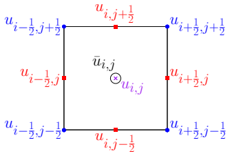
The central mechanism is the active flux semi-discretization itself: cell averages are advanced by a conservative finite-volume flux through Simpson's rule, while interface point values are advanced by local Lax-Friedrichs flux vector splitting with upwind one-sided differences; because point values are continuous across interfaces, no Riemann solver is needed. The Godunov-Powell source term $-\left(\nabla\cdot B\right)\Psi$, with $\Psi=(0,B_1,B_2,v\cdot B)^\top$, is discretized compactly: the cell-average source uses the $3\times3$ Gauss-Lobatto quadrature on the bi-parabolic reconstruction, and the point-value divergence is a central difference built on the same stencil. Positivity is carried by two limiters: a parametrized flux limiter that blends the high-order cell-average fluxes and source with the first-order positivity-preserving LLF scheme, and a scaling limiter for point values. The shock-suppression machinery is a sensor $\theta^s_{i+1/2,j}=\exp\left(-\kappa[(\varphi_1)(\varphi_2)+\varphi_3]\right)$ built from total-pressure jumps, velocity dilatation, and a new discrete $\nabla\cdot B$ term, which sets local blending coefficients for both fluxes and the source term.
What would settle it
A direct check would be to construct or randomly search for a set of admissible vertex states for which one vertex pressure is nonnegative only after radial shrinking, yet the coordinate-wise minimum rectangle is not contained in the pressure-admissible set; evaluating the limited scheme on that state should yield a negative-pressure cell average, contradicting the claimed guarantee. Short of that, a formal counterexample to the containment statement would settle the question, since the paper gives no proof of it.
Extended reading notes
Core claim
The central claim is that the active flux scheme with the LLF flux vector splitting and the Godunov-Powell source term is third-order accurate and positivity-preserving for both cell averages and point values, while keeping the discrete divergence under control. For the cell average, the source term is discretized by a $3\times3$ Gauss-Lobatto quadrature using the bi-parabolic reconstruction, and the flux is blended with the first-order positivity-preserving LLF flux through a parametrized flux limiter; for the point values, the flux derivative uses LLF splitting and the divergence is approximated by a central difference, with a scaling limiter enforcing admissibility. The paper further introduces a shock sensor that combines a total-pressure jump sensor, a velocity-dilatation sensor, and a new discrete magnetic-divergence term; the sensor's blending coefficient damps the high-order flux and source term near discontinuities. Numerical tests on two-dimensional problems, including smooth accuracy tests, the Orszag-Tang vortex, rotor, blast wave, shock-cloud interaction, and magnetized jets, are presented as evidence that the scheme retains third-order convergence, positivity, and stable divergence error over long times.
Load-bearing premise
In the cell-average limiter of Section 3.2, the pressure-positivity guarantee rests on an unproved geometric assertion: after radially shrinking each vertex of the parameter rectangle to make it pressure-admissible, the rectangle formed by the coordinate-wise minima of the shrunk vertices still lies inside the pressure-admissible set; if that containment fails, the blended cell average is not guaranteed to stay positive even though the numerical tests do.
Editorial extensions
If this is right
- The scheme attains third-order $\ell^1$ convergence on smooth two-dimensional tests, including a vortex whose central pressure drops to about $5.3\times10^{-12}$.
- With the PP limitings active, the scheme runs to completion on the Leblanc shock, rotor, blast-wave, shock-cloud, and high-Mach jet problems; without them, negative pressure appears within one step or shortly after.
- The Godunov-Powell source term, discretized as specified, controls divergence error: the two monitored discrete divergences grow slowly and reach a plateau in the Orszag-Tang test, and the rotor test shows distorted Mach contours when the source term is omitted from either the cell-average or the point-value update.
- The shock-sensor blending is applied locally rather than globally, so high-order resolution is retained in smooth regions while oscillations near strong discontinuities are damped.
- The scheme stays compact: the source-term discretizations for both cell averages and point values use only degrees of freedom in the current cell or on its edges, matching the stencil of the original active flux method.
Reading between the lines
- If the unproved rectangle-containment assertion fails, the scheme may still be numerically positivity-preserving; the paper's guarantee would weaken from a theorem to an empirical property, and a repairing argument would need to find a smaller or differently shaped admissible subset.
- The same two-step blending (source first, then flux) could plausibly transfer to three-dimensional MHD, where the additional direction enlarges the parameter rectangle but the convexity argument appears to require only more bookkeeping.
- The new magnetic-divergence term in the shock sensor could be reused as a standalone refinement indicator: regions where $\varphi_3$ is large mark places where the discrete divergence has not yet been advected away, which is exactly where a divergence-cleaning or mesh-refinement step would pay off.
- Because the cell-average blending is designed to keep mass conservation through unique interface fluxes, the method may be a useful building block for MHD codes that need strict conservation of mass but can tolerate the nonconservative momentum and energy updates introduced by the Godunov-Powell term.
Editorial analysis
A structured set of objections, weighed in public.
Referee Report
Summary. This paper proposes a positivity-preserving active flux (AF) scheme for the two-dimensional ideal MHD equations with the Godunov-Powell source term. The cell average is updated by a conservative finite volume formula, while the nonconservative source term is discretized by a 3x3 Gauss-Lobatto quadrature based on the in-cell bi-parabolic reconstruction; the point values are evolved by the LLF flux vector splitting from [25] with a central-difference discretization of the divergence in the source term. Positivity is enforced by blending the high-order AF update with the first-order LLF scheme whose PP property was proved in [58]: a parametrized flux limiter is constructed for the cell average and a scaling limiter for the point values. A new shock sensor involving total pressure, velocity divergence and magnetic-field divergence is used to damp oscillations through additional blending. Numerical experiments (smooth accuracy tests, Orszag-Tang, rotor, blast, shock-cloud interaction, and MHD jets) demonstrate third-order convergence, positivity, oscillation control, and control of the discrete divergence error.
Significance. If the central claims hold, the paper is a valuable contribution: it extends the compact active flux methodology to ideal MHD with a positivity guarantee and with a Godunov-Powell source discretization that does not enlarge the stencil. The use of the externally proved first-order LLF PP property [58] as the fallback scheme is methodologically sound, and the numerical test suite is substantial, including problems with very low pressure that would crash without the limiters. The evidence for third-order accuracy and for divergence control is convincing. The main weakness is that two load-bearing PP assertions are not proved in the manuscript: the geometric containment step in Section 3.2 and the direct applicability of Lemma 3.1 to the staggered face-centered point-value LLF updates in Section 3.3. Because the paper's headline property is 'positivity-preserving', these gaps must be closed before the claims can be taken as established. No code or data is provided, so numerical reproducibility cannot be independently assessed.
major comments (3)
- [Section 3.2] In Step (2) of the parametrized flux limiter, the paper asserts that the rectangle defined by Lambda_I = min_{k_I=1} B_{k,I} is 'a rectangular subset inside the convex polygon with vertices B_k'. This containment is load-bearing: the PP proof of U^{Lim,2}_{i,j}(theta) requires every theta in the box [0,Lambda_L] x [0,Lambda_R] x [0,Lambda_D] x [0,Lambda_U] to yield an admissible state. For arbitrary point sets the coordinate-wise minimum box is not contained in the convex hull (e.g., conv{(0,0),(1,100),(100,1)} contains neither (1,0) nor (0,1)); the special ray-scaling structure may rescue the claim, but no argument is given. The round-off fallback in Remark 4.1 does not address a structural overestimate of the admissible coefficients. Please add a proof (or a precise reference) that the constructed box lies in S_p, or modify the construction so that containment is explicit.
- [Section 3.3] The statement that the three first-order LLF schemes for the point values 'are PP according to Lemma 3.1' is not justified for the face-centered updates. For U_{i+1/2,j}, the y-direction stencil uses points at y_{j-1/2}, y_j and y_{j+1/2} with spacing Delta_y/2, while the source-term divergence uses a denominator 2 Delta_y; Lemma 3.1 is stated for cell averages on a uniform mesh with spacing Delta_x, Delta_y and a central source term evaluated at distance Delta_y from the cell center. A direct application is therefore not immediate, and the point-value PP property is part of Definition 3.1. Please provide a proof (for example, by representing the update as a convex combination of Lemma 3.1 updates on suitable sub-grids) and state the corresponding CFL condition, or restrict the PP claim to the cell average with a separate numerical justification for the point values.
- [Section 3.2, Step (1)] The formula theta_{i,j} = min(1, (p(U^{LLF}_{i,j}) - eps_p)/(p(U^{LLF}_{i,j}) - p(U^{src}_{i,j}))) is not valid when p(U^{src}_{i,j}) >= p(U^{LLF}_{i,j}): the fraction is then negative and the coefficient leaves [0,1]. In that case concavity of the pressure gives p(U^{Lim,1}_{i,j}) >= eps_p for every theta in [0,1], so the standard fix is to set theta = 1 when the denominator is non-positive. Please add this case distinction; as written, the source-blending step of the PP construction is incomplete.
minor comments (6)
- [Section 4 / Section 2] The numerical tests never state the CFL number or the time-step formula used. Since the PP property depends on the CFL condition in Lemma 3.1 and on analogous conditions for the point-value updates, please report the time-step control used in all examples.
- [Section 2.2] The discrete divergence values in equation (6) are labeled with indices (0,0), (0,1), ..., (2,2), while the quadrature points are labeled with l,m = 1,2,3. Please make the correspondence explicit to avoid confusion.
- [Example 4.2] The initial data for the Leblanc problem are listed as identical to those of the first Riemann problem in Example 4.1, with only the adiabatic index and final time changed. Please clarify whether this is intended and cite the specific Leblanc setup from [40] explicitly.
- [Section 3.4] The shock sensor strength kappa is chosen differently in nearly every test (kappa = 1, 2, 10, 50, 1000) and no sensitivity study is provided. Please comment on the sensitivity of the results to kappa and on how it should be selected in practice.
- [Section 3.3] In the formula for theta*_sigma, the denominator is written as rho(U^L_sigma) - rho(U^H_sigma); presumably U^{LLF}_sigma is intended. Please correct this typo.
- [Example 4.5] The phrase 'tapper function' should read 'taper function'.
Circularity Check
No circular reduction found; self-citations ([25], [3]) are not load-bearing, and the §3.2 geometric unproved lemma is a correctness gap rather than circularity.
full rationale
I walked the claimed derivation chain: the third-order AF cell-average update is a standard finite-volume/Simpson construction, and the point-value LLF-FVS update is taken from the authors' own [25], but it is an ingredient chosen by prior numerical evidence, not a parameter fitted to the present tests. The PP result is not circular: Lemma 3.1 (first-order LLF positivity with the Godunov-Powell source) is cited from the external Wu-Shu paper [58]; the parametrized flux limiter follows Xu [60] and Christlieb et al. [19,20]; the scaling limiter is Zhang-Shu [61]/Liu-Osher [41]. The authors' own [25] contributes the blending idea and the FVS discretization, but the blending target (first-order LLF) has an independent PP proof, so the self-citation is not load-bearing. Accuracy and PP are verified on independent smooth and shock benchmarks (Examples 4.1-4.8) rather than derived from fitted constants; the shock-sensor strength kappa is hand-set per test, but it is not fitted to the reported accuracy or positivity metrics, so it does not turn a demonstration into a prediction. I do flag one non-circular gap: in Section 3.2, the sentence 'Finally, let us find a rectangular subset inside the convex polygon with vertices B_{k_L,k_R,k_D,k_U} by Lambda_{I_{i,j},I} = min_{(k_L,k_R,k_D,k_U), k_I=1} B_{k_L,k_R,k_D,k_U,I}' asserts without proof that the coordinate-wise-minimum box lies in the pressure-admissible convex set; that geometric lemma is load-bearing for the guaranteed PP update, and the general claim is not self-evident. Remark 4.1's rounding fallback is an implementation safeguard, not a derivation step. The flagged gap is an omitted-proof/correctness risk, not an equivalence of the result to its inputs, so it does not raise the circularity score. The low score 2 is for the presence of minor self-citations in the construction, not for any circular reduction.
Assumptions & free parameters
free parameters (3)
- shock sensor strength kappa =
10, 50, 1000, 1, 2, 1, 1, 2 (per test in Examples 4.1-4.8)
- positivity floor and denominator regularizers =
10^-13 and 10^-40
- round-off rescue shrink factor =
2^m * 10^-8 with m=0..9
assumptions (6)
- domain assumption The Godunov-Powell source term modified MHD system is a valid formulation for divergence control.
- standard math The first-order LLF scheme with discrete Godunov-Powell source term is positivity-preserving (Lemma 3.1).
- standard math The admissible state set G is convex.
- standard math SSP-RK3 is a convex combination of forward Euler steps, so PP in forward Euler implies PP in the fully discrete scheme.
- domain assumption The bi-parabolic reconstruction and finite difference operators are third-order accurate and exact for bi-parabolic polynomials.
- ad hoc to paper The rectangle defined by coordinate-wise minima of the shrunken vertices lies in the pressure-admissible set S_p.
Cite this review
Pith. "Pith review of Active flux for ideal magnetohydrodynamics: A positivity-preserving scheme with the Godunov-Powell source term." pith.science (2026). https://pith.science/paper/KXKV3PKN
@misc{pith2026250604857,
  author       = {Pith},
  title        = {Pith review of: Active flux for ideal magnetohydrodynamics: A positivity-preserving scheme with the Godunov-Powell source term},
  year         = {2026},
  howpublished = {\url{https://pith.science/paper/KXKV3PKN}},
  note         = {Machine review of arXiv:2506.04857}
}
read the original abstract
The Active Flux (AF) is a compact, high-order finite volume scheme that allows more flexibility by introducing additional point value degrees of freedom at cell interfaces. This paper proposes a positivity-preserving (PP) AF scheme for solving the ideal magnetohydrodynamics, where the Godunov-Powell source term is employed to deal with the divergence-free constraint. For the evolution of the cell average, apart from the standard conservative finite volume method for the flux derivative, the nonconservative source term is built on the quadratic reconstruction in each cell, which maintains the compact stencil in the AF scheme. For the point value update, the local Lax-Friedrichs (LLF) flux vector splitting is adopted for the flux derivative, originally proposed in [Duan, Barsukow, and Klingenberg, SIAM Journal on Scientific Computing, 47(2), A811--A837, 2025], and a central difference is used to discretize the divergence in the source term. A parametrized flux limiter and a scaling limiter are presented to preserve the density and pressure positivity by blending the AF scheme with the first-order PP LLF scheme with the source term. To suppress oscillations, a new shock sensor considering the divergence error is proposed, which is used to compute the blending coefficients for the cell average. Several numerical tests are conducted to verify the third-order accuracy, PP property, and shock-capturing ability of the scheme. The key role of the Godunov-Powell source term and its suitable discretization in controlling divergence error is also validated.
Figures


Figures from the paper (9 more)


Reference graph
Works this paper leans on
-
[25]
J. Duan, W. Barsukow, and C. Klingenberg , Active flux methods for hyperbolic conservation laws -- flux vector splitting and bound-preservation , SIAM J. Sci. Comput., 47 (2025), pp. A811--A837, https://doi.org/10.1137/24M1658887
-
[58]
K. Wu and C.-W. Shu , Provably positive high-order schemes for ideal magnetohydrodynamics: Analysis on general meshes , Numer. Math., (2019), https://doi.org/10.1007/s00211-019-01042-w
-
[1]
R. Abgrall , A combination of residual distribution and the active flux formulations or a new class of schemes that can combine several writings of the same hyperbolic problem: application to the 1D Euler equationss , Commun. Appl. Math. Comput., 5 (2023), pp. 370--402, https://doi.org/10.1007/s42967-021-00175-w
-
[2]
R. Abgrall and W. Barsukow , Extensions of active flux to arbitrary order of accuracy , ESAIM: Math. Model. Numer. Anal., 57 (2023), pp. 991--1027, https://doi.org/10.1051/m2an/2023004
arXiv 2023
-
[3]
R. Abgrall, W. Barsukow, and C. Klingenberg , A semi-discrete active flux method for the Euler equations on Cartesian grids , J. Sci. Comput., 102 (2025), p. 36, https://doi.org/10.1007/s10915-024-02749-1
-
[4]
Bound preserving Point-Average-Moment PolynomiAl-interpreted (PAMPA) scheme: one-dimensional case
R. Abgrall, M. Jiao, Y. Liu, and K. Wu , Bound preserving Point-Average-Moment PolynomiAl-interpreted ( PAMPA ) scheme: O ne-dimensional case , Oct. 2024, https://doi.org/10.48550/arXiv.2410.14292
work page Pith review arXiv doi:10.48550/arxiv.2410.14292 2024
-
[5]
D. S. Balsara , Second-order-accurate schemes for magnetohydrodynamics with divergence-free reconstruction , Astrophys. J. Suppl. Ser., 151 (2004), p. 149, https://doi.org/10.1086/381377
doi:10.1086/381377 2004
-
[6]
D. S. Balsara , Self-adjusting, positivity preserving high order schemes for hydrodynamics and magnetohydrodynamics , J. Comput. Phys., 231 (2012), pp. 7504--7517, https://doi.org/10.1016/j.jcp.2012.01.032
Show all 62 references
-
[7]
D. S. Balsara and D. Spicer , Maintaining pressure positivity in magnetohydrodynamic simulations , J. Comput. Phys., 148 (1999), pp. 133--148, https://doi.org/10.1006/jcph.1998.6108
1999
-
[8]
D. S. Balsara and D. S. Spicer , A staggered mesh algorithm using high order Godunov fluxes to ensure solenoidal magnetic fields in magnetohydrodynamic simulations , J. Comput. Phys., 149 (1999), pp. 270--292, https://doi.org/10.1006/jcph.1998.6153
1999
-
[9]
Barsukow , The active flux scheme for nonlinear problems , J
W. Barsukow , The active flux scheme for nonlinear problems , J. Sci. Comput., 86 (2021), p. 3, https://doi.org/10.1007/s10915-020-01381-z
2021 doi
-
[10]
Barsukow and J
W. Barsukow and J. P. Berberich , A well-balanced active flux method for the shallow water equations with wetting and drying , Commun. Appl. Math. Comput., (2023), https://doi.org/10.1007/s42967-022-00241-x
2023 doi
-
[11]
Barsukow, J
W. Barsukow, J. P. Berberich, and C. Klingenberg , On the active flux scheme for hyperbolic PDEs with source terms , SIAM J. Sci. Comput., 43 (2021), pp. A4015--A4042, https://doi.org/10.1137/20M1346675
2021 doi
-
[12]
Barsukow, J
W. Barsukow, J. Hohm, C. Klingenberg, and P. L. Roe , The active flux scheme on Cartesian grids and its low Mach number limit , J. Sci. Comput., 81 (2019), pp. 594--622, https://doi.org/10.1007/s10915-019-01031-z
2019 doi
-
[13]
Bouchut, C
F. Bouchut, C. Klingenberg, and K. Waagan , A multiwave approximate Riemann solver for ideal MHD based on relaxation. I : Theoretical framework , Numer. Math., 108 (2007), pp. 7--42, https://doi.org/10.1007/s00211-007-0108-8
2007 doi
-
[14]
Bouchut, C
F. Bouchut, C. Klingenberg, and K. Waagan , A multiwave approximate Riemann solver for ideal MHD based on relaxation II : Numerical implementation with 3 and 5 waves , Numer. Math., 115 (2010), pp. 647--679, https://doi.org/10.1007/s00211-010-0289-4
2010 doi
-
[15]
J. U. Brackbill and D. C. Barnes , The effect of nonzero B on the numerical solution of the magnetohydrodynamic equations , J. Comput. Phys., 35 (1980), pp. 426--430, https://doi.org/10.1016/0021-9991(80)90079-0
1980 doi
-
[16]
Brio and C
M. Brio and C. C. Wu , An upwind differencing scheme for the equations of ideal magnetohydrodynamics , J. Comput. Phys., 75 (1988), pp. 400--422, https://doi.org/10.1016/0021-9991(88)90120-9
1988 doi
-
[17]
Chandrashekar and C
P. Chandrashekar and C. Klingenberg , Entropy stable finite volume scheme for ideal compressible MHD on 2- D Cartesian meshes , SIAM J. Numer. Anal., 54 (2016), pp. 1313--1340, https://doi.org/10.1137/15m1013626
2016 doi
-
[18]
Cheng, F
Y. Cheng, F. Li, J. Qiu, and L. Xu , Positivity-preserving DG and central DG methods for ideal MHD equations , J. Comput. Phys., 238 (2013), pp. 255--280, https://doi.org/10.1016/j.jcp.2012.12.019
2013 doi
-
[19]
A. J. Christlieb, X. Feng, D. C. Seal, and Q. Tang , A high-order positivity-preserving single-stage single-step method for the ideal magnetohydrodynamic equations , J. Comput. Phys., 316 (2016), pp. 218--242, https://doi.org/10.1016/j.jcp.2016.04.016
2016 doi
-
[20]
A. J. Christlieb, Y. Liu, Q. Tang, and Z. Xu , Positivity-preserving finite difference weighted ENO schemes with constrained transport for ideal magnetohydrodynamic equations , SIAM J. Sci. Comput., 37 (2015), pp. A1825--A1845, https://doi.org/10.1137/140971208
2015 doi
-
[21]
Chudzik, C
E. Chudzik, C. Helzel, and M. Lukáčová-Medvid’ová , Active flux methods for hyperbolic systems using the method of bicharacteristics , J. Sci. Comput., 99 (2024), p. 16, https://doi.org/10.1007/s10915-024-02462-z
2024 doi
-
[22]
Dai and P
W. Dai and P. R. Woodward , A simple finite difference scheme for multidimensional magnetohydrodynamical equations , J. Comput. Phys., 142 (1998), pp. 331--369, https://doi.org/10.1006/jcph.1998.5944
1998
-
[23]
Dedner, F
A. Dedner, F. Kemm, D. Kröner, C.-D. Munz, T. Schnitzer, and M. Wesenberg , Hyperbolic divergence cleaning for the MHD equations , J. Comput. Phys., 175 (2002), pp. 645--673, https://doi.org/10.1006/jcph.2001.6961
2002
-
[24]
Ding and K
S. Ding and K. Wu , A new discretely divergence-free positivity-preserving high-order finite volume method for ideal MHD equations , SIAM J. Sci. Comput., 46 (2024), pp. A50--A79, https://doi.org/10.1137/23m1562081
2024 doi
-
[26]
Ducros, V
F. Ducros, V. Ferrand, F. Nicoud, C. Weber, D. Darracq, C. Gacherieu, and T. Poinsot , Large-eddy simulation of the shock/turbulence interaction , J. Comput. Phys., 152 (1999), pp. 517--549, https://doi.org/10.1006/jcph.1999.6238
1999
-
[27]
C. R. Evans and J. F. Hawley , Simulation of magnetohydrodynamic flows: A constrained transport method , Astrophys. J., 332 (1988), p. 659, https://doi.org/10.1086/166684
1988 doi
-
[28]
Eymann and P
T. Eymann and P. Roe , Active flux schemes , in 49th AIAA Aerospace Sciences Meeting including the New Horizons Forum and Aerospace Exposition , Orlando, Florida, Jan. 2011, American Institute of Aeronautics and Astronautics, https://doi.org/10.2514/6.2011-382
2011 doi
-
[29]
Eymann and P
T. Eymann and P. Roe , Active flux schemes for systems , in 20th AIAA Computational Fluid Dynamics Conference, Fluid Dynamics and Co -located Conferences , American Institute of Aeronautics and Astronautics, June 2011, https://doi.org/10.2514/6.2011-3840
2011 doi
-
[30]
T. A. Eymann and P. L. Roe , Multidimensional active flux schemes , in 21st AIAA Computational Fluid Dynamics Conference, Fluid Dynamics and Co -located Conferences , American Institute of Aeronautics and Astronautics, June 2013, https://doi.org/10.2514/6.2013-2940
2013 doi
-
[31]
D. Fan , On the Acoustic Component of Active Flux Schemes for Nonlinear Hyperbolic Conservation Laws , thesis, University of Michigan, Ann Arbor, Michigan, 2017, http://deepblue.lib.umich.edu/handle/2027.42/140800
2017
-
[32]
Fan and P
D. Fan and P. L. Roe , Investigations of a new scheme for wave propagation , in 22nd AIAA Computational Fluid Dynamics Conference , American Institute of Aeronautics and Astronautics, 2015, https://doi.org/10.2514/6.2015-2449
2015 doi
-
[33]
T. A. Gardiner and J. M. Stone , An unsplit Godunov method for ideal MHD via constrained transport , J. Comput. Phys., 205 (2005), pp. 509--539, https://doi.org/10.1016/j.jcp.2004.11.016
2005 doi
-
[34]
S. K. Godunov , Symmetric form of the magnetohydrodynamic equation , Numer. Meth. Mech. Cont. Media, 1 (1972), pp. 26--34
1972
-
[35]
Helzel, D
C. Helzel, D. Kerkmann, and L. Scandurra , A new ADER method inspired by the active flux method , J. Sci. Comput., 80 (2019), pp. 1463--1497, https://doi.org/10.1007/s10915-019-00988-1
2019 doi
-
[36]
Jameson, W
A. Jameson, W. Schmidt, and E. Turkel , Solutions of the Euler equations by finite volume methods using Runge - Kutta time-stepping schemes , AIAA J., 1259 (1981)
1981
-
[37]
Janhunen , A positive conservative method for magnetohydrodynamics based on HLL and Roe methods , J
P. Janhunen , A positive conservative method for magnetohydrodynamics based on HLL and Roe methods , J. Comput. Phys., 160 (2000), pp. 649--661, https://doi.org/10.1006/jcph.2000.6479
2000
-
[38]
Li and C
F. Li and C. W. Shu , Locally divergence-free discontinuous Galerkin methods for MHD equations, magneto , J. Sci. Comput., 22--23 (2005), pp. 413--442, https://doi.org/10.1007/s10915-004-4146-4
2005 doi
-
[39]
F. Li, L. Xu, and S. Yakovlev , Central discontinuous Galerkin methods for ideal MHD equations with the exactly divergence-free magnetic field , J. Comput. Phys., 230 (2011), pp. 4828--4847, https://doi.org/10.1016/j.jcp.2011.03.006
2011 doi
-
[40]
Liu and K
M. Liu and K. Wu , Structure-preserving oscillation-eliminating discontinuous Galerkin schemes for ideal mhd equations: Locally divergence-free and positivity-preserving , J. Comput. Phys., 527 (2025), p. 113795, https://doi.org/10.1016/j.jcp.2025.113795
2025
-
[41]
Liu and S
X.-D. Liu and S. Osher , Nonoscillatory high order accurate self-similar maximum principle satisfying shock capturing schemes I , SIAM J. Numer. Anal., 33 (1996), pp. 760--779, https://doi.org/10.1137/0733038
1996 doi
-
[42]
Liu, C.-W
Y. Liu, C.-W. Shu, and M. P. Zhang , Entropy stable high order discontinuous Galerkin methods for ideal compressible MHD on structured meshes , J. Comput. Phys., 354 (2018), pp. 163--178, https://doi.org/10.1016/j.jcp.2017.10.043
2018 doi
-
[43]
Londrillo and L
P. Londrillo and L. Del Zanna , On the divergence-free condition in Godunov -type schemes for ideal magnetohydrodynamics: the upwind constrained transport method , J. Comput. Phys., 195 (2004), pp. 17--48, https://doi.org/10.1016/j.jcp.2003.09.016
2004 doi
-
[44]
Miyoshi and K
T. Miyoshi and K. Kusano , A multi-state HLL approximate riemann solver for ideal magnetohydrodynamics , J. Comput. Phys., 208 (2005), pp. 315--344, https://doi.org/10.1016/j.jcp.2005.02.017
2005 doi
-
[45]
S. A. Orszag and C.-M. Tang , Small-scale structure of two-dimensional magnetohydrodynamic turbulence , J. Fluid Mech., 90 (1979), pp. 129--143, https://doi.org/10.1017/S002211207900210X
1979 doi
-
[46]
Report 94-24, ICASE, NASA Langley, 1994
Powell , An approximate Riemann solver for magnetohydrodynamics (that works in more than one dimension) , Tech. Report 94-24, ICASE, NASA Langley, 1994
1994
-
[47]
K. G. Powell, P. L. Roe, T. J. Linde, T. I. Gombosi, and D. L. De Zeeuw , A solution-adaptive upwind scheme for ideal magnetohydrodynamics , J. Comput. Phys., 154 (1999), pp. 284--309, https://doi.org/10.1006/jcph.1999.6299
1999
-
[48]
Roe , Is discontinuous reconstruction really a good idea? , J
P. Roe , Is discontinuous reconstruction really a good idea? , J. Sci. Comput., 73 (2017), pp. 1094--1114, https://doi.org/10.1007/s10915-017-0555-z
2017 doi
-
[49]
Ryu and T
D. Ryu and T. Jones , Numerical magnetohydrodynamics in astrophysics: algorithm and tests for one-dimensional flow , Astrophys. J., 442 (1995), pp. 228--257, https://doi.org/10.1086/175437
1995 doi
-
[50]
J. M. Stone, T. A. Gardiner, P. Teuben, J. F. Hawley, and J. B. Simon , Athena: A new code for astrophysical mhd , Astrophys. J. Suppl. Ser., 178 (2008), pp. 137--177, https://doi.org/10.1086/588755
2008 doi
-
[51]
Tóth , The B =0 constraint in shock-capturing magnetohydrodynamics codes , J
G. Tóth , The B =0 constraint in shock-capturing magnetohydrodynamics codes , J. Comput. Phys., 161 (2000), pp. 605--652, https://doi.org/10.1006/jcph.2000.6519
2000
-
[52]
Van Leer , Towards the ultimate conservative difference scheme
B. Van Leer , Towards the ultimate conservative difference scheme. IV . A new approach to numerical convection , J. Comput. Phys., 23 (1977), pp. 276--299, https://doi.org/10.1016/0021-9991(77)90095-X
1977 doi
-
[53]
Waagan , A positive MUSCL - Hancock scheme for ideal magnetohydrodynamics , J
K. Waagan , A positive MUSCL - Hancock scheme for ideal magnetohydrodynamics , J. Comput. Phys., 228 (2009), pp. 8609--8626, https://doi.org/10.1016/j.jcp.2009.08.020
2009 doi
-
[54]
Waagan, C
K. Waagan, C. Federrath, and C. Klingenberg , A robust numerical scheme for highly compressible magnetohydrodynamics: Nonlinear stability, implementation and tests , J. Comput. Phys., 230 (2011), pp. 3331--3351, https://doi.org/10.1016/j.jcp.2011.01.026
2011 doi
-
[55]
A. R. Winters and G. J. Gassner , Affordable, entropy conserving and entropy stable flux functions for the ideal MHD equations , J. Comput. Phys., 304 (2016), pp. 72--108, https://doi.org/10.1016/j.jcp.2015.09.055
2016 doi
-
[56]
Wu , Positivity-preserving analysis of numerical schemes for ideal magnetohydrodynamics , SIAM J
K. Wu , Positivity-preserving analysis of numerical schemes for ideal magnetohydrodynamics , SIAM J. Numer. Anal., 56 (2018), pp. 2124--2147, https://doi.org/10.1137/18m1168017
2018 doi
-
[57]
Wu and C.-w
K. Wu and C.-w. Shu , A provably positive discontinuous Galerkin method for multidimensional ideal magnetohydrodynamics , SIAM J. Sci. Comput., 40 (2018), pp. B1302--B1329, https://doi.org/10.1137/18m1168042
2018 doi
-
[59]
Wu and H
K. Wu and H. Tang , Admissible state and physical constraints preserving schemes for relativistic magnetohydrodynamic equations , Math. Models Methods Appl. Sci., 27 (2017), pp. 1871--1928, https://doi.org/10.1142/S0218202517500348
2017 doi
-
[60]
Xu , Parametrized maximum principle preserving flux limiters for high order schemes solving hyperbolic conservation laws: O ne-dimensional scalar problem , Math
Z. Xu , Parametrized maximum principle preserving flux limiters for high order schemes solving hyperbolic conservation laws: O ne-dimensional scalar problem , Math. Comput., 83 (2014), pp. 2213--2238, https://doi.org/10.1090/S0025-5718-2013-02788-3
2014 doi
-
[61]
Zhang and C.-W
X. Zhang and C.-W. Shu , On positivity-preserving high order discontinuous Galerkin schemes for compressible Euler equations on rectangular meshes , J. Comput. Phys., 229 (2010), pp. 8918--8934, https://doi.org/10.1016/j.jcp.2010.08.016
2010 doi
-
[62]
write newline
" write newline "" before.all 'output.state := FUNCTION fin.entry add.period write newline FUNCTION new.block output.state before.all = 'skip after.block 'output.state := if FUNCTION not #0 #1 if FUNCTION and 'skip pop #0 if FUNCTION or pop #1 'skip if FUNCTION new.block.check...
Reviewed August 7, 2026 · model on record in the stance chip above.
Discussion (0). Sign in to comment.