REVIEW 4 major objections 6 minor 46 references
Equitable Discrimination in Survival Prediction: The Maximum Expected C-Index
T0 review · 4 major / 6 minor · reviewed 2026-08-07 · deepseek-v4-flash
Pith's one-line read A survival model's ranking power is capped by the expected C-Index of the true hazard model, not by 1.
desk verdict The subpopulation C-index is a useful descriptive tool, but the oracle-based upper bound is computed from observed survival times, so the headline 0.75 ECI and the discrimination ratios are not valid. read the letter →
The pith
A machine-rendered reading of the paper's core claim, the machinery that carries it, and where it could break.
The reading
What carries the argument
The key object is the pairwise win probability $p_{ij} = P(T_i > T_j) = h_j/(h_i+h_j)$, where $h_i$ is the time-independent hazard multiplier of member $i$ under proportional hazards. This identity carries the argument because it lets the expected C-Index be written as a sum of terms that the true ranking maximizes termwise, independently of the baseline survival function. In practice the bound is computed by recovering empirical hazard multipliers $h^*_i$ from an estimated baseline survival function and observed event times, then forming the model $M^*$ whose expected C-Index is the upper bound.
What would settle it
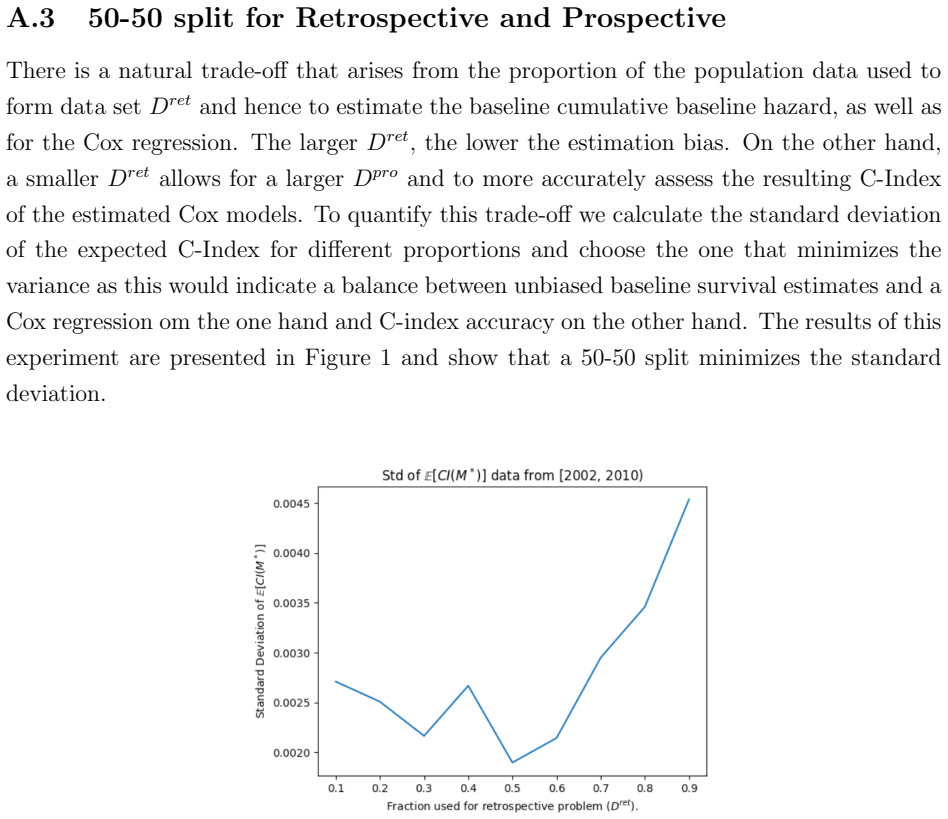
Simulate survival times from a known proportional-hazards model with a Weibull baseline and two strong predictors, compute the ECI ceiling from the true hazard multipliers, then fit a Cox model that omits one predictor; if its observed C-Index exceeds the ECI ceiling across repeated random 50/50 splits, the empirical version of the bound fails as a universal ceiling.
Extended reading notes
Core claim
Proposition 2 is the load-bearing result: for any prediction model $\hat M$, $E[CI(\hat M)] \le E[CI(M)]$, where $M$ is the true model generated by the proportional-hazards survival functions; and in uncensored complete-case data $E[CI(M)] \le E[CI^U(M)]$. The proof rests on Proposition 1, which gives the pairwise probability that member $i$ outlives member $j$ as $p_{ij} = h_j/(h_i+h_j)$, a quantity independent of the baseline hazard. Because the true model maximizes concordance in expectation, scores that look low against 1 can be near the attainable ceiling when judged against ECI. In the UNOS/OPTN case study the ceiling for ten-year death-censored graft survival is about 0.75, and a Cox model scoring 0.61-0.62 has a discrimination ratio of roughly 37-52 percent—closing about half the gap between chance and the boundary. For subpopulations, the SUBECI ceilings barely differ across Asian, Black, Hispanic/Latino, and White patients, while the SUBCIs differ significantly, which the paper reads as evidence that the Cox model is ethnically biased.
Load-bearing premise
The load-bearing premise is that the hazard multipliers $h^*_i$ used to compute the ceiling are unbiased estimates of the true hazards, which requires the proportional-hazards model to be correctly specified with no important predictors omitted; if the model is misspecified, the computed ECI is not a ceiling every other model must respect.
Editorial extensions
If this is right
- Reported C-Index values should be read against ECI rather than against 1: a 0.61 score on ten-year death-censored graft survival lies about halfway between 0.5 and the 0.75 ceiling, not in the lower-middle range toward 1.
- The discrimination ratio $DR = (CI - 0.5)/(ECI - 0.5)$ gives a normalized performance measure; values around 0.37-0.52 in this case study quantify how much of the attainable ranking power the Cox model captures.
- Because subpopulation ceilings are similar while observed SUB C-Indices differ significantly, the gap between SUBCI and SUBECI can flag biased models even when the overall C-Index looks acceptable.
- Undersampling to balance ethnic subpopulations raises most subpopulation C-Indices but does not remove the differences, so data imbalance alone does not explain the bias.
- The upper bound applies to any model whose implied survival functions satisfy proportional hazards, so machine-learning survival models can be compared with Cox models against the same ECI benchmark.
Reading between the lines
- Testable extension: apply the same ECI and SUBECI machinery to other allocation-driven survival problems, such as liver or heart transplant, credit-default, or customer-churn survival, to see whether subpopulation ceilings stay nearly flat while model scores diverge; the kidney-transplant equity conclusion would be strengthened if the pattern generalizes.
- Implicit consequence: if ECI is a tight ceiling, then the room for improvement in a Cox model is exactly the gap between its discrimination ratio and 1; a ranking-oriented machine-learning model that surpasses the Cox DR without exceeding ECI would demonstrate that the ceiling is reachable in practice.
- Neighbouring problem: the same pairwise win-probability identity suggests closed-form expected-concordance bounds for other C-Index variants that the paper lists as future work; deriving those would turn each variant into a comparable benchmark rather than an unnormalized score.
- Design implication: because SUBECI ceilings are nearly equal while SUBCIs differ, a fairness intervention could aim to equalize subpopulation discrimination ratios rather than raw C-Indices; this is a target the paper gestures at but does not itself implement.
Editorial analysis
A structured set of objections, weighed in public.
Referee Report
Summary. The paper proposes a new upper bound, the expected C-Index (ECI), for the C-Index of survival prediction models under proportional hazards, together with a subpopulation C-Index (SUBCI) and a discrimination ratio (DR). The theoretical claims are given as Proposition 1 (pairwise concordance probability for proportional hazards) and Proposition 2 (the expected C-Index of the true model is an upper bound for any prediction model, with a tighter bound in the uncensored case). The methods are applied to UNOS kidney-transplant data to estimate ECI for death-censored graft survival, to compare overall and subpopulation C-Indices, and to argue that a standard Cox model is ethnically biased. The paper claims ECI around 0.75, making a C-Index of ~0.61 close to half the gap to the upper bound.
Significance. If the central theorem were correct, the ECI would provide a practically useful benchmark for survival prediction, and the subpopulation extension would be a valuable contribution to fairness evaluation in medical prediction. The paper has concrete strengths: Proposition 1 is correct under the stated assumptions; the definition of SUBCI is a meaningful and apparently novel way to measure discrimination within subpopulations; the case study uses a large registry dataset and the code is publicly available. However, the central upper-bound claim (Proposition 2) is not valid for censored data, and the empirical ECI is computed from a data-dependent oracle construction rather than from the true hazards. These flaws are load-bearing: they affect the headline ECI value, the discrimination ratios, and the ethnic-bias conclusions. The contribution is therefore not yet established.
major comments (4)
- [Section 2.3, Proposition 2] The proof of the first inequality in Proposition 2 is incorrect, and the statement is false for censored data. The problem appears in the line: 'By definition of M, Mij = 1 implies hj/(\tilde h_i + h_j) > 1/2 > \tilde h_i/(\tilde h_i + h_j).' This implication is not valid: from Mij=1 we have hi < hj, but \tilde h_i can exceed h_j when i is censored, so hj/(\tilde h_i+h_j) may be less than 1/2. Moreover, the comparison with the \hat M_j i term is wrong: when \hat M predicts j>i, the relevant probability is E[A_ji] = hi/(\tilde h_j + hi), not \tilde h_i/(\tilde h_i+h_j). A concrete counterexample: two members, i censored at time 0 (so \tilde T_i=0) and j uncensored, with hi=1, hj=2. The true model M predicts i>j (since E[Ti]>E[Tj]), but E[A_ij]=0 and E[A_ji]=1, so E[CI(M)]=0 while any model that predicts j>i has E[CI]=1. This violates Eq. (14). Since all subsequent results (DR, SUBECI, and the case-study conclusions) rely on Proposition 2 as an upper bound, the censored-data bound is not established.
- [Section 3, construction of M*] The empirical ECI is not a valid upper bound because it is computed from oracle hazard rates. The text states: 'For Dret, we can calculate unbiased hazard rates h*_i satisfying E[T*_i] = Ti' and then forms M* with survival functions S*_i(t)=[S0(t)]^{h*_i}. These h*_i are functions of the realized outcome Ti, not the population hazard parameters hi used in Proposition 2; accordingly the paper observes that CI(M*)=1 in Dret. Proposition 2 applies to the true model M whose hazards are fixed population parameters, not to a model that sees the outcomes. Replacing hi by h*_i = g(Ti) can inflate the bound: in a homogeneous population the true PH bound is 0.5, but the construction yields approximately 0.75 for exponential survival. Therefore the ECI values of about 0.75 reported in Tables 1 and 2, the discrimination ratios in Tables 3 and 4, and the claim that a C-Index of 0.61 'closes almost half the gap' are not supported by the theory.
- [Section 2.2 and Definition 3, notational inconsistency] The definition of Aij is inconsistent across the manuscript. In Section 2.2, Aij is defined for censored data as Aij = 1 if \tilde T_i > T_j (with \tilde T_i the observed censored/event time), and this is the form used in the proof of Proposition 2 and in the ECI expressions. Definition 3, however, restates Aij = 1 if Ti > Tj, using the unobserved event time, and the surrounding text returns to uncensored notation without cleaning up. This ambiguity makes it difficult to verify which expression is used in the case study; it also affects the interpretation of K and the weights in Section 2.4. The authors should standardize notation and make explicit whether all Aij in the censored setting are based on \tilde T_i.
- [Section 3, transfer of the bound from Dret to Dpro] The statement 'if both Dret and Dpro are large enough random samples from the same original data set, any maximum expected C-Index calculated for Dret also applies to Dpro' is an additional assumption that is not justified. Even if the oracle-hazard issue were resolved, the h*_i are defined on the realized event times in Dret, and their distribution in Dpro is not shown to be the same. A formal argument for the transferability of the upper bound is needed; without it, the case-study numbers compare a Dret-derived bound to a Dpro-derived C-Index in an unsupported way. This issue is separate from the misspecification concern raised in the text.
minor comments (6)
- [Section 1, Introduction] The abstract and introduction treat 'survival' and 'time to event' interchangeably; the paper should state explicitly that longer survival corresponds to later event time, to avoid confusion with the proportional-hazards direction.
- [Section 2.3, Definition 4] Definition 4 uses E[Aij] without specifying the probability space; it would be clearer to write E[Aij] as a function of the hazards and censoring distribution, and to define the expectation over the joint distribution of (Ti, Di).
- [Section 4, Tables 1-4] The tables report 95% confidence intervals over 30 random splits. The text should state whether these intervals account for within-split correlation between the model C-Index and the ECI bound; the current description is insufficient for a reader to judge the significance of the differences.
- [Section 3, Definition 9] The discrimination ratio DR subtracts 0.5 in both numerator and denominator; this is a valid rescaling only if E[CI(M*)] > 0.5, which is not proven for the censored case. Please add a condition or justification.
- [Appendix A.2, Predictor table] Table 6 lists 'Donor's Age' twice; one entry should be removed or replaced by the intended variable (e.g., donor age squared).
- [General] The paper contains several typographical errors (e.g., 'C-index' vs 'C-Index' inconsistently; 'shows present an upperbound' in the Conclusion; 'the narrow confidence interval show' in Section 4). A careful proofreading pass is needed.
Circularity Check
Empirical ECI bound is computed from an outcome-calibrated oracle model, so the headline 0.75 bound and the discrimination ratios are fitted quantities rather than independent PH upper bounds.
-
fitted input called prediction
[Section 3, paragraph beginning 'After the transfer of an unbiased baseline survival function...']
"For Dret, we can calculate unbiased hazard rates h∗ i satisfying E[T ∗ i ] = Ti, i= 1, . . . , m. Being unbiased, the h∗ i can be used to form a prediction model M ∗ with survival functions S∗ i (t) = [S0(t)]h∗ i . Now, because M ∗ ij = 1 if Aij = 1 for every pair i, jin P ret, CI (M ∗) = 1 in Dret. Moreover, E[CI (M ∗)] is an upper bound for the E[CI ( ˆM )] attainable by any prediction model ˆM on Dret and Dpro."
Proposition 2 bounds E[CI(ˆM)] by the expected C-Index of the true model M, whose hazards h_i are fixed population parameters. The empirical implementation instead defines h*_i by solving E[T*_i] = T_i, i.e., by calibrating each hazard to the observed outcome. Because E[T] decreases in the hazard, this forces M*'s predicted ordering to match the observed event order, which is why CI(M*)=1 on Dret. E[CI(M*)] is therefore a function of the realized T_i values, not an upper bound derived from the true PH model. In a homogeneous population the true bound is 0.5, yet this construction can produce values near 0.75, so the reported ECI and SUBECI bounds are fitted, outcome-dependent quantities, not independent upper limits.
-
fitted input called prediction
[Definition 9 and Abstract]
"DR( ˆM , M∗) = CI ( ˆM ) − 0.5 / E[CI (M ∗)] − 0.5 . (23) ... With an ECI of 0.75 for 10-year survival, the new upperbound is well below 1. A C-Index performance around 0.61 or slightly above as commonly reported in literature and replicated in this study therefore closes almost half of the gap between the ECI and the 0.5 threshold."
The discrimination ratio and the 'closes almost half the gap' claim normalize the observed C-Index by E[CI(M*)]-0.5. Since E[CI(M*)] is inflated by the outcome-calibrated construction of M*, the denominator is not the true-model bound from Proposition 2 but a fitted benchmark. The ratio CI(ˆM)-0.5 over an outcome-fit denominator does not measure how much of the PH-achievable discrimination is captured; it measures performance against an oracle that has seen the event times. Thus the headline numerical conclusion depends on the same fitted values used to define the benchmark.
full rationale
The theoretical contribution in Proposition 1 and Proposition 2 is not circular: the proof derives P(T_i > T_j) = h_j/(h_i + h_j) from the PH assumption and then shows that the true model's expected C-Index dominates any other model's expected C-Index purely from the ordering of hazards. That argument is self-contained and does not depend on the case study. The circularity enters in the empirical application. Section 3 replaces the true hazards h_i of Proposition 2 with h*_i chosen so that E[T*_i] equals each observed event time T_i. This is an outcome-calibrated oracle model, and the paper itself notes that CI(M*)=1 on Dret. Calling these hazards 'unbiased' does not make M* the true PH model; it makes M* a function of the realized outcomes over which the C-Index and its bound are computed. Consequently, the reported ECI of about 0.75, the SUBECI bounds, and the discrimination ratios are not upper bounds for models under the PH assumption but quantities forced by the h* construction. The ethnic-bias comparison of SUBCIs against these inflated SUBECI bounds inherits the same problem. The paper contains self-citations, but they are not the load-bearing source of circularity; the reduction is by construction in the empirical ECI. Score 6 reflects that the central empirical claim reduces to a fit, while the theorem itself remains independent.
Assumptions & free parameters
free parameters (4)
- Cox model regression coefficients =
Not reported individually
- Baseline survival function S0(t) =
Estimated nonparametrically via Breslow/Kaplan-Meier
- Split proportion (0.5) =
0.5
- Perturbation epsilon for ties =
Small, unspecified
assumptions (5)
- domain assumption True hazard functions are proportional: h_i(t) = h_i * h_0(t)
- domain assumption Independent right censoring
- ad hoc to paper Correct model specification: the Cox covariate set captures the true hazards
- ad hoc to paper Unbiasedness of h*_i: E[T*_i] = T_i
- domain assumption Distinct event times
Cite this review
Pith. "Pith review of Equitable Discrimination in Survival Prediction: The Maximum Expected C-Index." pith.science (2026). https://pith.science/paper/G22HOEQE
@misc{pith2026250605592,
  author       = {Pith},
  title        = {Pith review of: Equitable Discrimination in Survival Prediction: The Maximum Expected C-Index},
  year         = {2026},
  howpublished = {\url{https://pith.science/paper/G22HOEQE}},
  note         = {Machine review of arXiv:2506.05592}
}
read the original abstract
The C-Index measures the discrimination performance of survival prediction models. C-Index scores are often well below the upperbound of 1 that represents perfect prediction and closer to 0.5 as achieved by random prediction. Our first objective is to provide a tighter C-Index upperbound for proportional hazards models. Our second research objective is to measure discrimination performance for subpopulations, also relative to subpopulation specific upperbounds. We present the expected C-Index (ECI) as a tight upperbound for proportional hazards models. Moreover, we define the subpopulation C-Index (SUBCI) and a sub-population specific expected C-Index (SUBECI). The metrics are applied to predict death censored graft survival (DCGF) after deceased donor kidney transplant in the US with a Cox model using standard donor (KDPI), patient (EPTS), and (Class 1) mismatch predictors. With an ECI of 0.75 for 10-year survival, the new upperbound is well below 1. A C-Index performance around 0.61 or slightly above as commonly reported in literature and replicated in this study therefore closes almost half of the gap between the ECI and the 0.5 threshold. SUBECIs don't vary significantly from the overall ECI but there are substantial and significant differences among the SUBCIs. Extending this upperbound and C-Index to subpopulations enables to identify differences in discrimination upperbounds across subpopulations and in prediction model biases. A standard Cox model for DCGF in the US can be ethnically biased.
Figures
Reference graph
Works this paper leans on
-
[1]
Regression models and life-tables
David R Cox. Regression models and life-tables. Journal of the Royal Statistical Society: Series B (Methodological), 34(2):187–202, 1972
1972
-
[2]
Regression modelling strategies for improved prognostic prediction
Frank E Harrell Jr, Kerry L Lee, Robert M Califf, David B Pryor, and Robert A Rosati. Regression modelling strategies for improved prognostic prediction. Statistics in medicine, 3(2):143–152, 1984
work page 1984
-
[3]
Time to default in credit scoring using survival analysis: a benchmark study
Lore Dirick, Gerda Claeskens, and Bart Baesens. Time to default in credit scoring using survival analysis: a benchmark study. Journal of the Operational Research Society , 68(6):652–665, 2017
work page 2017
-
[4]
Prognostic modeling of predictive maintenance with survival analysis for mobile work equipment
Zhen Yang, Juho Kanniainen, Tomi Krogerus, and Frank Emmert-Streib. Prognostic modeling of predictive maintenance with survival analysis for mobile work equipment. Scientific Reports, 12(1):8529, 2022
work page 2022
-
[5]
Gary S Collins, Johannes B Reitsma, Douglas G Altman, and Karel GM Moons. Trans- parent reporting of a multivariable prediction model for individual prognosis or diagnosis (tripod) the tripod statement. Circulation, 131(2):211–219, 2015
work page 2015
-
[6]
Probast: a tool to assess the risk of bias and applicability of prediction model studies
Robert F Wolff, Karel GM Moons, Richard D Riley, Penny F Whiting, Marie Westwood, Gary S Collins, Johannes B Reitsma, Jos Kleijnen, Sue Mallett, and PROBAST Group†. Probast: a tool to assess the risk of bias and applicability of prediction model studies. Annals of internal medicine , 170(1):51–58, 2019
work page 2019
-
[7]
Machine learning for survival analysis: A survey
Ping Wang, Yan Li, and Chandan K Reddy. Machine learning for survival analysis: A survey. ACM Computing Surveys (CSUR) , 51(6):1–36, 2019
work page 2019
-
[8]
Deep learning for survival analysis: a review
Simon Wiegrebe, Philipp Kopper, Raphael Sonabend, Bernd Bischl, and Andreas Ben- der. Deep learning for survival analysis: a review. Artificial Intelligence Review , 57(3):65, 2024
work page 2024
Show all 46 references
-
[9]
The comparative performance of models predicting patient and graft survival after kidney transplantation: A systematic review
Joris van de Klundert, Francisco Perez-Galarce, Marcelo Olivares, Liset Pengel, and Annelies de Weerd. The comparative performance of models predicting patient and graft survival after kidney transplantation: A systematic review. Transplantation Reviews, page 100934, 2025
2025
-
[10]
Verification of forecasts expressed in terms of probability
Glenn W Brier. Verification of forecasts expressed in terms of probability. Monthly weather review, 78(1):1–3, 1950. 21
1950
-
[11]
Assessment and comparison of prognostic classification schemes for survival data
Erika Graf, Claudia Schmoor, Willi Sauerbrei, and Martin Schumacher. Assessment and comparison of prognostic classification schemes for survival data. Statistics in medicine, 18(17-18):2529–2545, 1999
1999
-
[12]
Signal detection theory and psychophysics , volume 1
David Marvin Green, John A Swets, et al. Signal detection theory and psychophysics , volume 1. Wiley New York, 1966
1966
-
[13]
Receiver-operating characteristic (roc) plots: a fundamental evaluation tool in clinical medicine
Mark H Zweig and Gregory Campbell. Receiver-operating characteristic (roc) plots: a fundamental evaluation tool in clinical medicine. Clinical chemistry, 39(4):561–577, 1993
1993
-
[14]
Assessing the performance of prediction models: a framework for traditional and novel measures
Ewout W Steyerberg, Andrew J Vickers, Nancy R Cook, Thomas Gerds, Mithat Go- nen, Nancy Obuchowski, Michael J Pencina, and Michael W Kattan. Assessing the performance of prediction models: a framework for traditional and novel measures. Epidemiology, 21(1):128–138, 2010
2010
-
[15]
A com- prehensive risk quantification score for deceased donor kidneys: the kidney donor risk index
Panduranga S Rao, Douglas E Schaubel, Mary K Guidinger, Kenneth A Andreoni, Robert A Wolfe, Robert M Merion, Friedrich K Port, and Randall S Sung. A com- prehensive risk quantification score for deceased donor kidneys: the kidney donor risk index. Transplantation, 88(2):231–236, 2009
2009
-
[16]
Nicholas Hartman, Sehee Kim, Kevin He, and John D Kalbfleisch. c. Statistics in medicine, 42(13):2179–2190, 2023
2023
-
[17]
Machine learning to predict transplant outcomes: helpful or hype? a national cohort study
Sunjae Bae, Allan B Massie, Brian S Caffo, Kyle R Jackson, and Dorry L Segev. Machine learning to predict transplant outcomes: helpful or hype? a national cohort study. Transplant International, 33(11):1472–1480, 2020
2020
-
[18]
Large-scale benchmark study of survival prediction methods using multi- omics data
Moritz Herrmann, Philipp Probst, Roman Hornung, Vindi Jurinovic, and Anne-Laure Boulesteix. Large-scale benchmark study of survival prediction methods using multi- omics data. Briefings in bioinformatics , 22(3):bbaa167, 2021
2021
-
[19]
Ensuring fairness in machine learning to advance health equity.Annals of internal medicine, 169(12):866–872, 2018
Alvin Rajkomar, Michaela Hardt, Michael D Howell, Greg Corrado, and Marshall H Chin. Ensuring fairness in machine learning to advance health equity.Annals of internal medicine, 169(12):866–872, 2018
2018
-
[20]
Gianfrancesco, Suzanne Tamang, Jinoos Yazdany, and Gabriela Schmajuk
Milena A. Gianfrancesco, Suzanne Tamang, Jinoos Yazdany, and Gabriela Schmajuk. Potential Biases in Machine Learning Algorithms Using Electronic Health Record Data. JAMA Internal Medicine , 178(11):1544–1547, 11 2018. 22
2018
-
[21]
Risk of bias in studies on prediction models developed using supervised machine learning techniques: systematic review
Constanza L Andaur Navarro, Johanna AA Damen, Toshihiko Takada, Steven WJ Nij- man, Paula Dhiman, Jie Ma, Gary S Collins, Ram Bajpai, Richard D Riley, Karel GM Moons, et al. Risk of bias in studies on prediction models developed using supervised machine learning techniques: sy...
2021
-
[22]
Predictably unequal: understanding and address- ing concerns that algorithmic clinical prediction may increase health disparities
Jessica K Paulus and David M Kent. Predictably unequal: understanding and address- ing concerns that algorithmic clinical prediction may increase health disparities. NPJ digital medicine, 3(1):99, 2020
2020
-
[23]
The effectiveness, equity and explainability of health service resource allocation-with applications in kidney transplantation & family planning
Joris Van De Klundert, Harwin De Vries, Francisco P´ erez Galarce, Nieves Valdes, and Felipe Simon. The effectiveness, equity and explainability of health service resource allocation-with applications in kidney transplantation & family planning. Frontiers in Health Services, 5...
2025
-
[24]
Statistical modeling: Regression, survival analysis, and time series analysis
Lawrence Leemis. Statistical modeling: Regression, survival analysis, and time series analysis. N/A, 2023
2023
-
[25]
Empirical likelihood in survival analysis
Gang Li, Runze Li, and Mai Zhou. Empirical likelihood in survival analysis. In Contem- porary Multivariate Analysis And Design Of Experiments: In Celebration of Professor Kai-Tai Fang’s 65th Birthday , pages 337–349. World Scientific, 2005
2005
-
[26]
Statistical models based on counting processes
Per K Andersen, Ornulf Borgan, Richard D Gill, and Niels Keiding. Statistical models based on counting processes. Springer Science & Business Media, 2012
2012
-
[27]
Two-sided bias bound of the kaplan-meier estimator
M Zhou. Two-sided bias bound of the kaplan-meier estimator. Probability theory and related fields, 79(2):165–173, 1988
1988
-
[28]
The bias of kaplan-meier integrals
Winfried Stute. The bias of kaplan-meier integrals. Scandinavian Journal of Statistics , pages 475–484, 1994
1994
-
[29]
The kidney allocation system
John J Friedewald, Ciara J Samana, Bertram L Kasiske, Ajay K Israni, Darren Stewart, Wida Cherikh, and Richard N Formica. The kidney allocation system. Surgical Clinics, 93(6):1395–1406, 2013
2013
-
[30]
A guide to calculating and interpreting the estimated post-transplant survival (epts) score used in the kidney allocation system (kas)
OPTN. A guide to calculating and interpreting the estimated post-transplant survival (epts) score used in the kidney allocation system (kas). Kidney, 2, 2012
2012
-
[31]
A guide to calculating and interpreting the kidney donor profile index (kdpi)
OPTN. A guide to calculating and interpreting the kidney donor profile index (kdpi). Accesed at https://optnpilot. unos. org/media/1512/guide to calculating interpreting kdpi. pdf on , 8, 2018. 23
2018
-
[32]
Long-term kidney transplant graft survival—making progress when most needed
Emilio D Poggio, Joshua J Augustine, Susana Arrigain, Daniel C Brennan, and Jesse D Schold. Long-term kidney transplant graft survival—making progress when most needed. American journal of transplantation , 21(8):2824–2832, 2021
2021
-
[33]
The statistical sign test
Wilfrid J Dixon and Alexander M Mood. The statistical sign test. Journal of the American Statistical Association, 41(236):557–566, 1946
1946
-
[34]
On a test of whether one of two random variables is stochastically larger than the other
Henry B Mann and Donald R Whitney. On a test of whether one of two random variables is stochastically larger than the other. The annals of mathematical statistics , pages 50–60, 1947
1947
-
[35]
Multical- ibration: Calibration for the (computationally-identifiable) masses
Ursula H´ ebert-Johnson, Michael Kim, Omer Reingold, and Guy Rothblum. Multical- ibration: Calibration for the (computationally-identifiable) masses. In International Conference on Machine Learning , pages 1939–1948. PMLR, 2018
1939
-
[36]
Prediction performance and fairness heterogeneity in cardiovascular risk models
Uri Kartoun, Shaan Khurshid, Bum Chul Kwon, Aniruddh P Patel, Puneet Batra, Anthony Philippakis, Amit V Khera, Patrick T Ellinor, Steven A Lubitz, and Kenney Ng. Prediction performance and fairness heterogeneity in cardiovascular risk models. Scientific Reports, 12(1):12542, 2022
2022
-
[37]
Bias and unfairness in machine learning models: a systematic review on datasets, tools, fairness metrics, and identification and mitigation methods
Tiago P Pagano, Rafael B Loureiro, Fernanda VN Lisboa, Rodrigo M Peixoto, Guil- herme AS Guimar˜ aes, Gustavo OR Cruz, Maira M Araujo, Lucas L Santos, Marco AS Cruz, Ewerton LS Oliveira, et al. Bias and unfairness in machine learning models: a systematic review on datasets, to...
2023
-
[38]
Fairness in predicting cancer mortality across racial subgroups
Teja Ganta, Arash Kia, Prathamesh Parchure, Min-heng Wang, Melanie Besculides, Madhu Mazumdar, and Cardinale B Smith. Fairness in predicting cancer mortality across racial subgroups. JAMA Network Open , 7(7):e2421290–e2421290, 2024
2024
-
[39]
Effect of human leukocyte antigen compatibility on kidney graft survival: comparative analysis of two decades
Gerhard Opelz and Bernd D¨ ohler. Effect of human leukocyte antigen compatibility on kidney graft survival: comparative analysis of two decades. Transplantation, 84(2):137– 143, 2007
2007
-
[40]
Health disparities and health equity: concepts and measurement
Paula Braveman. Health disparities and health equity: concepts and measurement. Annual review of public health , 27(1):167–194, 2006
2006
-
[41]
What is health equity? Behavioral science & policy , 4(1):1–14, 2018
Paula Braveman, Elaine Arkin, Tracy Orleans, Dwayne Proctor, Julia Acker, and Alonzo Plough. What is health equity? Behavioral science & policy , 4(1):1–14, 2018. 24
2018
-
[42]
Eliminating transplant waiting time inequities–with an application to kidney allocation in the usa
Joris Van de Klundert, Liana van der Hagen, and Aniek Markus. Eliminating transplant waiting time inequities–with an application to kidney allocation in the usa. European Journal of Operational Research, 297(3):977–985, 2022
2022
-
[43]
Optn/srtr 2022 annual data report: kidney
Krista L Lentine, Jodi M Smith, Grace R Lyden, Jonathan M Miller, Thomas G Dolan, Keighly Bradbrook, Lindsay Larkin, Kayla Temple, Dzhuliyana K Handarova, Saman- tha Weiss, et al. Optn/srtr 2022 annual data report: kidney. American Journal of Transplantation, 24(2):S19–S118, 2024
2022
-
[44]
On ranking in survival analysis: Bounds on the concordance index
Harald Steck, Balaji Krishnapuram, Cary Dehing-Oberije, Philippe Lambin, and Vikas C Raykar. On ranking in survival analysis: Bounds on the concordance index. Advances in neural information processing systems , 20, 2007
2007
-
[45]
On the c-statistics for evaluating overall adequacy of risk prediction procedures with censored survival data
Hajime Uno, Tianxi Cai, Michael J Pencina, Ralph B D’Agostino, and Lee-Jen Wei. On the c-statistics for evaluating overall adequacy of risk prediction procedures with censored survival data. Statistics in medicine , 30(10):1105–1117, 2011
2011
-
[46]
A time-dependent discrimination index for survival data
Laura Antolini, Patrizia Boracchi, and Elia Biganzoli. A time-dependent discrimination index for survival data. Statistics in medicine , 24(24):3927–3944, 2005. 25 9 Tables Table 1: Expected C-Index vs actual C-Index for multiple years of transplants. The numbers in parenthese...
2005
Reviewed August 7, 2026 · model on record in the stance chip above.
Discussion (0). Sign in to comment.