REVIEW 3 major objections 5 minor 61 references
NAT: Neural Acoustic Transfer for Interactive Scenes in Real Time
T0 review · 3 major / 5 minor · reviewed 2026-08-07 · deepseek-v4-flash
Pith's one-line read A per-scene neural field predicts acoustic transfer maps for moving, resized, or re-materialized objects in a few milliseconds, making real-time dynamic sound rendering practical.
desk verdict A solid, genuinely useful method paper whose central claim survives scrutiny; the main weakness is an unproven singularity treatment in the data-generation pipeline, which is addressable and not fatal. read the letter →
The pith
A machine-rendered reading of the paper's core claim, the machinery that carries it, and where it could break.
The reading
What carries the argument
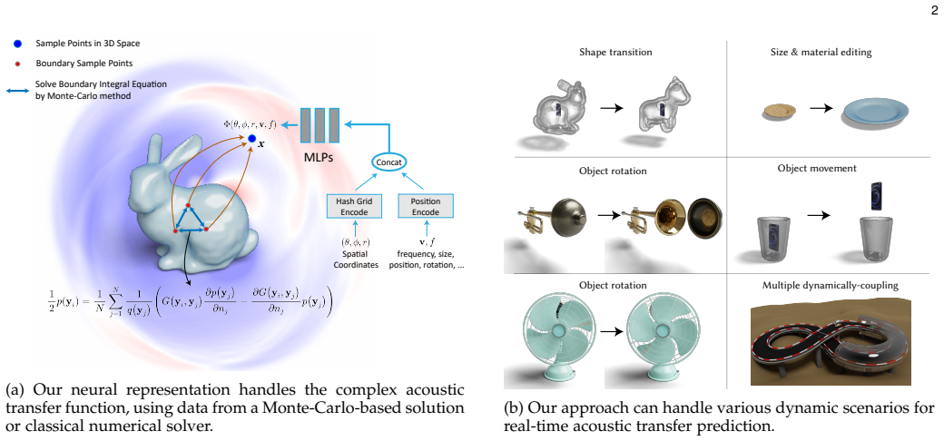
The machinery is the neural FFAT map, a continuous function $\Phi(\theta, \phi, r, v, f) = \mathrm{MLP}(G(\theta, \phi, r), P(v), P(f))$, where $G$ is a multi-resolution hash grid in spherical coordinates and $P$ is sinusoidal positional encoding. The hash grid supplies high-frequency spatial detail, the positional encoding lets a single network span ranges of frequency and scene conditions, and the MLP combines them into transfer values. Training data come from two solvers: a CUDA-accelerated boundary element method (BEM) for high precision, and a Monte-Carlo BEM approximation (BEM-MC) that replaces mesh quadrature with Poisson-disk boundary sampling plus a local singularity treatment, used for smooth Neumann scenes.
What would settle it
Run BEM-MC and standard BEM on a sphere with a known analytic radiation solution and a deliberately curved, well-resolved mesh; if the FFAT-map error of BEM-MC grows with surface curvature or does not shrink as Poisson-disk sample count increases, the neglected gradient integral is biasing the solver, and NAT inherits that bias.
Extended reading notes
Core claim
The paper's central claim is that a single neural network per scene can absorb the full variation of the acoustic transfer function over a continuous family of scene configurations. The network maps listener coordinates in a spherical hash grid plus condition parameters (position, rotation, size, material, shape proxy) and frequency through a small MLP to the far-field acoustic transfer map, so that at inference the expensive boundary-element solve is replaced by one forward pass. In validation, the predicted FFAT maps reach SNR 9.9–17.4 dB and SSIM 0.81–0.93 against BEM ground truth, while a 60-mode material and size edit takes about 2 ms and dynamic-scene transfer masks for 30 s of audio take 1–4 ms, several orders of magnitude faster than the prior neural method and with higher reported precision.
Load-bearing premise
The training-data pipeline rests on the assumption that a certain singular term in the boundary integral — the gradient of the Green's function integrated over a tiny disk around the evaluation point — is exactly zero because the radius vector is perpendicular to the surface normal; that is only exactly true at the center of a flat tangent disk, and the paper gives no error bound for curved surfaces.
Editorial extensions
If this is right
- A trained NAT model makes material and size editing of modal sound objects interactive: new material and size settings produce FFAT maps for all modes in about 2 ms, so a designer can hear the change live.
- Dynamic scenes with moving sources and resonating cavities, such as a phone moving in and out of a cup, can render a full acoustic transfer mask for 30 seconds of audio in 1–4 ms.
- Because the neural fit averages over nearby condition samples, NAT can report higher SSIM than the Monte-Carlo solver that produced its training data, meaning network inference acts as a variance reducer.
- The per-scene cost is roughly an hour of precomputation, about five minutes of training, and around one megabyte of model storage, so it is practical to replace stored transfer data with a small network.
Reading between the lines
- The same conditioning formulation could be extended to listener position and global environment state, effectively yielding a parameterized room impulse response; the paper stops at object-conditioned transfer rather than full room acoustics.
- Because the method trains a fresh network for each scene, it does not yet generalize to unseen scenes; a latent-space or multi-scene version would be the natural next step the paper leaves implicit.
- The reported SNR range (roughly 10–17 dB) suggests the target is audible plausibility rather than exact wave physics, so a listening study would be the right test of whether the accuracy actually matters perceptually.
- BEM-MC's sensitivity to the discarded gradient singularity could be probed directly by comparing against analytic radiation solutions on curved objects; if bias appears, NAT trained on BEM-MC inherits it.
Editorial analysis
A structured set of objections, weighed in public.
Referee Report
Summary. The paper proposes NAT, a per-scene implicit neural representation of acoustic transfer maps parameterized by listener position, frequency, and scene condition variables such as position, rotation, size, material, and shape. Training data are generated either by a CUDA-accelerated boundary element method (BEM) or by a proposed Monte-Carlo-based BEM approximation (BEM-MC) for smooth Neumann problems. The authors report 1-4 ms inference for 30 s audio, SNR 9.9-17.4 dB and SSIM 0.81-0.93 against BEM, and large speedups over NeuralSound, BEM, BEM-MC, and FDTD. The central claim is that, over a parameterized family of scene configurations, NAT predicts acoustic transfer in real time with accuracy close to BEM.
Significance. If the claims hold, the paper addresses a real bottleneck in interactive audio: making acoustic transfer editable and evaluable in real time for dynamically varying scenes. The empirical comparison is substantial: Tables 1, 2, and 4 include BEM, BEM-MC, NeuralSound, and NAT under controlled conditions, and Table 5 reports practical model sizes and inference times. The paper also honestly discloses that NAT can exceed its own training-data generator in SSIM, and attributes this to variance reduction, which is a reasonable and testable explanation. The experimental protocol is described in enough detail to be reproduced, and the speed-accuracy tradeoffs are reported clearly. The main weakness is theoretical: the BEM-MC singularity treatment in Eq. (13) is not derived or bounded, and since BEM-MC supplies most of the dynamic-scene training data, this gap propagates into the central claim.
major comments (3)
- [Sec. 4.2, Eq. (13)] The neglect of the Green's-function-gradient integral over the small disk is not justified for curved surfaces. The perpendicularity of r to n_y holds only at the disk center on a flat tangent plane; on a smooth curved surface r·n_y = O(ρ^2/R), so ∂r/∂n_y = O(ρ/R), and the omitted contribution is O(ε/R)p(y_i). The standard principal-value jump of the boundary integral does not vanish in general, and the manuscript supplies no bound in terms of ε, curvature, and wavenumber k. The pointer in Sec. 4.1.1 ('please refer to Section 6 for technical detail') is also unsatisfied, because Section 6 is the validation section rather than a derivation. Since BEM-MC is the training-data generator for the phone-cup scene and all extensive dynamic scenes (Tables 2, 4, 5; Figs. 3-6), any systematic bias in this term is inherited by NAT. Please provide the missing derivation and error bound, or empirically quantify the term by comparing BEM-MC solutions with and without the disk contribution on representative curved geometries.
- [Sec. 4.2, Eqs. (9)-(12)] The small-disk radius ε is a free parameter that is never specified or linked to the Poisson-disk sampling distance. The one-point estimate in Eq. (12) is dimensionally consistent but is a leading-order asymptotic approximation, not a standard N=1 Monte Carlo estimator of the disk integral (the area factor π ε^2 does not appear); the O(ε^2) and k-dependent error terms are not quantified. Because ε controls the magnitude of both the retained term in Eq. (12) and the neglected term in Eq. (13), a stated selection rule and a sensitivity study (e.g., varying ε at a fixed sample count) are needed to make the BEM-MC predictions reproducible and trustworthy.
- [Sec. 7, Table 5] For the six extensive scenes in Fig. 6, the paper reports only spectrograms and inference times; no SNR/SSIM or other accuracy metric against BEM or BEM-MC is given. These scenes include morphing geometry and multiple coupled sound sources, which are qualitatively more complex than the plate and phone-cup validations. The statement that NAT 'accurately captures' acoustic transfer across all these scenarios is therefore not directly supported by quantitative evidence. Adding at least one held-out quantitative validation for a morphing-shape or coupled-source scene would strengthen the generality of the central claim.
minor comments (5)
- [Sec. 6.3.1] The sentence 'The comparison of time cost and average precision ... is presented in Table 1' should refer to Table 4, which contains the 8-mode BEM-MC experiment; Table 1 reports the 60-mode BEM-based experiment.
- [Sec. 5.1 vs Sec. 7] The phone displacement range is stated as 0-0.3 m in Sec. 5.1 and as 0-0.2 m in Sec. 7; please reconcile the two descriptions.
- [Sec. 4.1.1, Eq. (7)] The symbol N is used both for the number of Monte Carlo samples in Eq. (7) and for the single-sample approximation in Eq. (12); using a distinct symbol (e.g., M_s) would avoid confusion.
- [Sec. 6.2] The statement that BEM-MC 'surpasses' CUDA-accelerated BEM is based on qualitative FFAT images in Fig. 8; please provide a quantitative metric for the analytical test cases to support this claim.
- [Sec. 8] The limitations paragraph mentions untuned hyperparameters and limited scene parameters, but does not mention the reliance on the unproven BEM-MC singularity treatment or the fact that only amplitude (not phase) is modeled; both are relevant caveats for the reported accuracy.
Circularity Check
No significant circularity: NAT is trained on BEM-generated labels and independently validated against BEM ground truth on held-out cases.
full rationale
The central claim of the paper is that a per-scene neural network, NAT, can predict acoustic transfer maps under varying conditions (position, rotation, size, material, shape) in milliseconds. The training labels come from either CUDA-accelerated BEM or BEM-MC, and the evaluation is performed against BEM as an external ground truth on held-out cases (Tables 1, 2, and 4; Figs. 2-4 and 9). This is standard supervised function approximation, not a fitted parameter renamed as a prediction: the network is not optimized against the test-time BEM solutions it is compared with. The reported cases where NAT surpasses its own BEM-MC training data in SSIM are explicitly disclosed as variance reduction and are cross-checked against BEM in the same tables, so they do not constitute a circular student-beats-teacher argument. The only self-citation of note is the authors' prior work NeuralSound [11], which is used as a comparison baseline rather than as load-bearing justification for NAT's accuracy; the comparison is external and quantified. The paper does contain an omitted technical derivation in Section 4.1.1/4.2: Eq. (13) sets the singular gradient integral to zero using a perpendicularity argument whose validity is conditional, and the promised reference to 'Section 6 for technical detail' points to a validation section rather than a derivation. This is a correctness and numerical-accuracy risk inherited by BEM-MC training data, but it is not circularity: it is an unproven approximation, not an equation that reduces to its own input or a claim justified only by self-citation. Therefore, no load-bearing circularity is present, and the appropriate circularity score is 0.
Assumptions & free parameters
free parameters (5)
- small-disk radius epsilon =
not reported
- Poisson disk sample count M =
1000, 2000, 4000
- spatial sample points per condition =
10,000
- network hyperparameters =
4x128 MLP; 4 hash levels at 8^3 to 64^3; feature length 4; 6 positional-encoding frequencies
- evaluation radius range =
1.5 to 3 times the scene bounding-box radius
assumptions (6)
- standard math Standard boundary element and Burton-Miller boundary integral equation theory (Eq. 6)
- ad hoc to paper The integral of the Green's function gradient over the small disk around the collocation point vanishes (Eq. 13)
- ad hoc to paper One-point Monte-Carlo estimate of the singular disk integral (Eq. 12)
- domain assumption Sufficiently smooth boundary for the local disk approximation
- domain assumption Neural network variance reduction makes BEM-MC data adequate for training
- domain assumption Helmholtz scaling: acoustic transfer depends on frequency times size
Cite this review
Pith. "Pith review of NAT: Neural Acoustic Transfer for Interactive Scenes in Real Time." pith.science (2026). https://pith.science/paper/YOLGWEBD
@misc{pith2026250606190,
  author       = {Pith},
  title        = {Pith review of: NAT: Neural Acoustic Transfer for Interactive Scenes in Real Time},
  year         = {2026},
  howpublished = {\url{https://pith.science/paper/YOLGWEBD}},
  note         = {Machine review of arXiv:2506.06190}
}
read the original abstract
Previous acoustic transfer methods rely on extensive precomputation and storage of data to enable real-time interaction and auditory feedback. However, these methods struggle with complex scenes, especially when dynamic changes in object position, material, and size significantly alter sound effects. These continuous variations lead to fluctuating acoustic transfer distributions, making it challenging to represent with basic data structures and render efficiently in real time. To address this challenge, we present Neural Acoustic Transfer, a novel approach that utilizes an implicit neural representation to encode precomputed acoustic transfer and its variations, allowing for real-time prediction of sound fields under varying conditions. To efficiently generate the training data required for the neural acoustic field, we developed a fast Monte-Carlo-based boundary element method (BEM) approximation for general scenarios with smooth Neumann conditions. Additionally, we implemented a GPU-accelerated version of standard BEM for scenarios requiring higher precision. These methods provide the necessary training data, enabling our neural network to accurately model the sound radiation space. We demonstrate our method's numerical accuracy and runtime efficiency (within several milliseconds for 30s audio) through comprehensive validation and comparisons in diverse acoustic transfer scenarios. Our approach allows for efficient and accurate modeling of sound behavior in dynamically changing environments, which can benefit a wide range of interactive applications such as virtual reality, augmented reality, and advanced audio production.
Figures


Figures from the paper (7 more)


Reference graph
Works this paper leans on
-
[1]
Scanning physical interaction behavior of 3d objects,
D. K. Pai, K. v. d. Doel, D. L. James, J. Lang, J. E. Lloyd, J. L. Rich- mond, and S. H. Yau, “Scanning physical interaction behavior of 3d objects,” in Proceedings of the 28th annual conference on Computer graphics and interactive techniques , 2001, pp. 87–96
work page 2001
-
[2]
Synthesizing sounds from rigid-body simulations,
J. F. O’Brien, C. Shen, and C. M. Gatchalian, “Synthesizing sounds from rigid-body simulations,” in Proceedings of the 2002 ACM SIGGRAPH/Eurographics symposium on Computer animation , 2002, pp. 175–181
work page 2002
-
[3]
D. L. James, J. Barbi ˇc, and D. K. Pai, “Precomputed acoustic transfer: output-sensitive, accurate sound generation for geomet- rically complex vibration sources,” ACM T ransactions on Graphics (Proceedings of SIGGRAPH 2006) , vol. 25, no. 3, pp. 987–995, 2006
work page 2006
-
[4]
Harmonic shells: a practical nonlinear sound model for near-rigid thin shells,
J. N. Chadwick, S. S. An, and D. L. James, “Harmonic shells: a practical nonlinear sound model for near-rigid thin shells,” ACM T ransactions on Graphics (Proceedings of SIGGRAPH 2009) , vol. 28, no. 5, pp. 1–10, 2009
work page 2009
-
[5]
The boundary element method in acoustics: A survey,
S. Kirkup, “The boundary element method in acoustics: A survey,” Applied Sciences, vol. 9, no. 8, p. 1642, 2019
work page 2019
-
[6]
Interactive acoustic transfer approx- imation for modal sound,
D. Li, Y. Fei, and C. Zheng, “Interactive acoustic transfer approx- imation for modal sound,” ACM T ransactions on Graphics (TOG) , vol. 35, no. 1, pp. 1–16, 2015
work page 2015
-
[8]
S. Hadadan, S. Chen, and M. Zwicker, “Neural radiosity,” ACM T ransactions on Graphics (TOG), vol. 40, no. 6, pp. 1–11, 2021
work page 2021
-
[10]
tiny-cuda-nn,
T. M ¨uller, “tiny-cuda-nn,” 4 2021. [Online]. Available: https: //github.com/NVlabs/tiny-cuda-nn
2021
Show all 61 references
-
[11]
Neuralsound: Learning-based modal sound synthesis with acoustic transfer,
X. Jin, S. Li, G. Wang, and D. Manocha, “Neuralsound: Learning-based modal sound synthesis with acoustic transfer,” ACM T rans. Graph. , vol. 41, no. 4, jul 2022. [Online]. Available: https://doi.org/10.1145/3528223.3530184
2022
-
[12]
Toward high-quality modal contact sound,
C. Zheng and D. L. James, “Toward high-quality modal contact sound,” in ACM SIGGRAPH 2011 papers , 2011, pp. 1–12
2011
-
[13]
Rigid-body fracture sound with precomputed sound- banks,
——, “Rigid-body fracture sound with precomputed sound- banks,” in ACM SIGGRAPH 2010 papers , 2010, pp. 1–13
2010
-
[14]
Eigenmode compression for modal sound models,
T. R. Langlois, S. S. An, K. K. Jin, and D. L. James, “Eigenmode compression for modal sound models,” ACM T ransactions on Graphics (Proceedings of SIGGRAPH 2014) , vol. 33, no. 4, Aug. 2014
2014
-
[15]
Syncopation: Interactive synthesis-coupled sound propagation,
A. Rungta, C. Schissler, R. Mehra, C. Malloy, M. Lin, and D. Manocha, “Syncopation: Interactive synthesis-coupled sound propagation,” IEEE transactions on visualization and computer graph- ics, vol. 22, no. 4, pp. 1346–1355, 2016
2016
-
[16]
Kleinpat: Optimal mode conflation for time-domain precomputation of acoustic transfer,
J.-H. Wang and D. L. James, “Kleinpat: Optimal mode conflation for time-domain precomputation of acoustic transfer,”ACM T rans- actions on Graphics (Proceedings of SIGGRAPH 2019) , vol. 38, no. 4, pp. 122:1–122:12, Jul. 2019
2019
-
[17]
Nerf: Representing scenes as neural radiance fields for view synthesis,
B. Mildenhall, P . P . Srinivasan, M. Tancik, J. T. Barron, R. Ra- mamoorthi, and R. Ng, “Nerf: Representing scenes as neural radiance fields for view synthesis,” Communications of the ACM , vol. 65, no. 1, pp. 99–106, 2021
2021
-
[18]
Implicit neural representations with periodic activation func- tions,
V . Sitzmann, J. Martel, A. Bergman, D. Lindell, and G. Wetzstein, “Implicit neural representations with periodic activation func- tions,” Advances in neural information processing systems , vol. 33, pp. 7462–7473, 2020
2020
-
[19]
Fourier features let networks learn high frequency functions in low dimensional domains,
M. Tancik, P . Srinivasan, B. Mildenhall, S. Fridovich-Keil, N. Raghavan, U. Singhal, R. Ramamoorthi, J. Barron, and R. Ng, “Fourier features let networks learn high frequency functions in low dimensional domains,” Advances in Neural Information Process- ing Systems, vol. 33, ...
2020
-
[20]
Efficient geometry-aware 3d generative adversarial networks,
E. R. Chan, C. Z. Lin, M. A. Chan, K. Nagano, B. Pan, S. De Mello, O. Gallo, L. J. Guibas, J. Tremblay, S. Khamis et al. , “Efficient geometry-aware 3d generative adversarial networks,” in Proceed- ings of the IEEE/CVF Conference on Computer Vision and Pattern Recognition, 202...
2022
-
[21]
Tensorf: Tensorial ra- diance fields,
A. Chen, Z. Xu, A. Geiger, J. Yu, and H. Su, “Tensorf: Tensorial ra- diance fields,” in European Conference on Computer Vision. Springer, 2022, pp. 333–350
2022
-
[22]
Plenoxels: Radiance fields without neural net- works,
S. Fridovich-Keil, A. Yu, M. Tancik, Q. Chen, B. Recht, and A. Kanazawa, “Plenoxels: Radiance fields without neural net- works,” in Proceedings of the IEEE/CVF Conference on Computer Vision and Pattern Recognition , 2022, pp. 5501–5510
2022
-
[23]
Acorn: Adaptive coordinate networks for neural scene representation,
J. N. Martel, D. B. Lindell, C. Z. Lin, E. R. Chan, M. Monteiro, and G. Wetzstein, “Acorn: Adaptive coordinate networks for neural scene representation,” arXiv preprint arXiv:2105.02788 , 2021
2021 arXiv
-
[24]
Mip-nerf: A multiscale represen- tation for anti-aliasing neural radiance fields,
J. T. Barron, B. Mildenhall, M. Tancik, P . Hedman, R. Martin- Brualla, and P . P . Srinivasan, “Mip-nerf: A multiscale represen- tation for anti-aliasing neural radiance fields,” in Proceedings of the IEEE/CVF International Conference on Computer Vision , 2021, pp. 5855–5864
2021
-
[25]
Ref-nerf: Structured view-dependent appearance for neural radiance fields,
D. Verbin, P . Hedman, B. Mildenhall, T. Zickler, J. T. Barron, and P . P . Srinivasan, “Ref-nerf: Structured view-dependent appearance for neural radiance fields,” in 2022 IEEE/CVF Conference on Com- puter Vision and Pattern Recognition (CVPR) . IEEE, 2022, pp. 5481– 5490
2022
-
[26]
Occupancy networks: Learning 3d reconstruction in 15 function space,
L. Mescheder, M. Oechsle, M. Niemeyer, S. Nowozin, and A. Geiger, “Occupancy networks: Learning 3d reconstruction in 15 function space,” in Proceedings of the IEEE/CVF conference on com- puter vision and pattern recognition , 2019, pp. 4460–4470
2019
-
[27]
Deepsdf: Learning continuous signed distance functions for shape representation,
J. J. Park, P . Florence, J. Straub, R. Newcombe, and S. Love- grove, “Deepsdf: Learning continuous signed distance functions for shape representation,” in Proceedings of the IEEE/CVF conference on computer vision and pattern recognition , 2019, pp. 165–174
2019
-
[28]
Convolutional occupancy networks,
S. Peng, M. Niemeyer, L. Mescheder, M. Pollefeys, and A. Geiger, “Convolutional occupancy networks,” in Computer Vision–ECCV 2020: 16th European Conference, Glasgow, UK, August 23–28, 2020, Proceedings, Part III 16 . Springer, 2020, pp. 523–540
2020
-
[29]
Neus: Learning neural implicit surfaces by volume rendering for multi-view reconstruction,
P . Wang, L. Liu, Y. Liu, C. Theobalt, T. Komura, and W. Wang, “Neus: Learning neural implicit surfaces by volume rendering for multi-view reconstruction,” arXiv preprint arXiv:2106.10689 , 2021
2021 arXiv
-
[30]
Learning gradient fields for shape generation,
R. Cai, G. Yang, H. Averbuch-Elor, Z. Hao, S. Belongie, N. Snavely, and B. Hariharan, “Learning gradient fields for shape generation,” in Computer Vision–ECCV 2020: 16th European Conference, Glasgow, UK, August 23–28, 2020, Proceedings, Part III 16 . Springer, 2020, pp. 364–381
2020
-
[31]
Bsp-net: Generating compact meshes via binary space partitioning,
Z. Chen, A. Tagliasacchi, and H. Zhang, “Bsp-net: Generating compact meshes via binary space partitioning,” in Proceedings of the IEEE/CVF Conference on Computer Vision and Pattern Recognition , 2020, pp. 45–54
2020
-
[32]
Learning implicit fields for generative shape modeling,
Z. Chen and H. Zhang, “Learning implicit fields for generative shape modeling,” in Proceedings of the IEEE/CVF Conference on Computer Vision and Pattern Recognition , 2019, pp. 5939–5948
2019
-
[33]
Pointflow: 3d point cloud generation with continuous normalizing flows,
G. Yang, X. Huang, Z. Hao, M.-Y. Liu, S. Belongie, and B. Har- iharan, “Pointflow: 3d point cloud generation with continuous normalizing flows,” in Proceedings of the IEEE/CVF international conference on computer vision , 2019, pp. 4541–4550
2019
-
[34]
Geometry processing with neural fields,
G. Yang, S. Belongie, B. Hariharan, and V . Koltun, “Geometry processing with neural fields,” Advances in Neural Information Processing Systems, vol. 34, pp. 22 483–22 497, 2021
2021
-
[35]
Generative neural articulated radiance fields,
A. Bergman, P . Kellnhofer, W. Yifan, E. Chan, D. Lindell, and G. Wetzstein, “Generative neural articulated radiance fields,” Ad- vances in Neural Information Processing Systems , vol. 35, pp. 19 900– 19 916, 2022
2022
-
[36]
Neural articulated ra- diance field,
A. Noguchi, X. Sun, S. Lin, and T. Harada, “Neural articulated ra- diance field,” in Proceedings of the IEEE/CVF International Conference on Computer Vision, 2021, pp. 5762–5772
2021
-
[37]
A level set theory for neural implicit evolution under explicit flows,
I. Mehta, M. Chandraker, and R. Ramamoorthi, “A level set theory for neural implicit evolution under explicit flows,” in European Conference on Computer Vision . Springer, 2022, pp. 711–729
2022
-
[38]
Implicit neural spatial representations for time-dependent pdes,
H. Chen, R. Wu, E. Grinspun, C. Zheng, and P . Y. Chen, “Implicit neural spatial representations for time-dependent pdes,” in Inter- national Conference on Machine Learning . PMLR, 2023, pp. 5162– 5177
2023
-
[39]
Neural caches for monte carlo partial differential equation solvers,
Z. Li, G. Yang, X. Deng, C. De Sa, B. Hariharan, and S. Marschner, “Neural caches for monte carlo partial differential equation solvers,” in SIGGRAPH Asia 2023 Conference Papers , 2023, pp. 1– 10
2023
-
[40]
Synthesis of musical instrument sounds: Physics-based modeling or machine learning,
S. H. Hawley, V . Chatziiannou, and A. Morrison, “Synthesis of musical instrument sounds: Physics-based modeling or machine learning,” Phys. T oday, vol. 16, no. 1, pp. 20–28, 2020
2020
-
[41]
A survey on deep learning for symbolic music generation: Representations, algorithms, evaluations, and challenges,
S. Ji, X. Yang, and J. Luo, “A survey on deep learning for symbolic music generation: Representations, algorithms, evaluations, and challenges,” ACM Computing Surveys , 2023
2023
-
[42]
Deep-modal: real- time impact sound synthesis for arbitrary shapes,
X. Jin, S. Li, T. Qu, D. Manocha, and G. Wang, “Deep-modal: real- time impact sound synthesis for arbitrary shapes,” in Proceedings of the 28th ACM International Conference on Multimedia , 2020, pp. 1171–1179
2020
-
[43]
Fast acoustic scattering using convolutional neural networks,
Z. Fan, V . Vineet, H. Gamper, and N. Raghuvanshi, “Fast acoustic scattering using convolutional neural networks,” in ICASSP 2020- 2020 IEEE International Conference on Acoustics, Speech and Signal Processing (ICASSP). IEEE, 2020, pp. 171–175
2020
-
[44]
Machine-learning-based estimation and rendering of scattering in virtual reality,
V . Pulkki and U. P . Svensson, “Machine-learning-based estimation and rendering of scattering in virtual reality,” The Journal of the Acoustical Society of America , vol. 145, no. 4, pp. 2664–2676, 2019
2019
-
[45]
Ir-gan: Room impulse response generator for far-field speech recognition,
A. Ratnarajah, Z. Tang, and D. Manocha, “Ir-gan: Room impulse response generator for far-field speech recognition,” arXiv preprint arXiv:2010.13219, 2020
2010 arXiv
-
[46]
Learning acoustic scat- tering fields for dynamic interactive sound propagation,
Z. Tang, H.-Y. Meng, and D. Manocha, “Learning acoustic scat- tering fields for dynamic interactive sound propagation,” in 2021 IEEE Virtual Reality and 3D User Interfaces (VR) . IEEE, 2021, pp. 835–844
2021
-
[47]
Learning neural acoustic fields,
A. Luo, Y. Du, M. Tarr, J. Tenenbaum, A. Torralba, and C. Gan, “Learning neural acoustic fields,” Advances in Neural Information Processing Systems, vol. 35, pp. 3165–3177, 2022
2022
-
[48]
Acoustic classification and optimization for multi-modal rendering of real-world scenes,
C. Schissler, C. Loftin, and D. Manocha, “Acoustic classification and optimization for multi-modal rendering of real-world scenes,” IEEE transactions on visualization and computer graphics , vol. 24, no. 3, pp. 1246–1259, 2017
2017
-
[49]
Scene-aware audio rendering via deep acoustic analysis,
Z. Tang, N. J. Bryan, D. Li, T. R. Langlois, and D. Manocha, “Scene-aware audio rendering via deep acoustic analysis,” IEEE transactions on visualization and computer graphics , vol. 26, no. 5, pp. 1991–2001, 2020
1991
-
[50]
Some continuous monte carlo methods for the dirichlet problem,
M. E. Muller, “Some continuous monte carlo methods for the dirichlet problem,” The Annals of Mathematical Statistics , pp. 569– 589, 1956
1956
-
[51]
Monte carlo geometry processing: A grid-free approach to pde-based methods on volumetric do- mains,
R. Sawhney and K. Crane, “Monte carlo geometry processing: A grid-free approach to pde-based methods on volumetric do- mains,” ACM T ransactions on Graphics, vol. 39, no. 4, 2020
2020
-
[52]
Pharr, W
M. Pharr, W. Jakob, and G. Humphreys, Physically based rendering: From theory to implementation . MIT Press, 2023
2023
-
[53]
Adam: A method for stochastic optimiza- tion,
D. P . Kingma and J. Ba, “Adam: A method for stochastic optimiza- tion,” in ICLR (Poster), 2015
2015
-
[54]
Automatic differ- entiation in pytorch,
A. Paszke, S. Gross, S. Chintala, G. Chanan, E. Yang, Z. DeVito, Z. Lin, A. Desmaison, L. Antiga, and A. Lerer, “Automatic differ- entiation in pytorch,” in NIPS-W, 2017
2017
-
[55]
Bempp-cl: A fast python based just-in-time compiling boundary element library
T. Betcke and M. W. Scroggs, “Bempp-cl: A fast python based just-in-time compiling boundary element library.” Journal of Open Source Software, vol. 6, no. 59, p. 2879, 2021
2021
-
[56]
A prac- tical walk-on-boundary method for boundary value problems,
R. Sugimoto, T. Chen, Y. Jiang, C. Batty, and T. Hachisuka, “A prac- tical walk-on-boundary method for boundary value problems,” ACM T rans. Graph., vol. 42, no. 4, jul 2023
2023
-
[57]
Walk on stars: A grid-free monte carlo method for pdes with neumann boundary conditions,
R. Sawhney, B. Miller, I. Gkioulekas, and K. Crane, “Walk on stars: A grid-free monte carlo method for pdes with neumann boundary conditions,” ACM T rans. Graph., vol. 42, no. 4, jul 2023. [Online]. Available: https://doi.org/10.1145/3592398
2023 doi
-
[58]
Parallel poisson disk sampling with spectrum analysis on surfaces,
J. Bowers, R. Wang, L.-Y. Wei, and D. Maletz, “Parallel poisson disk sampling with spectrum analysis on surfaces,” ACM T ransactions on Graphics (TOG) , vol. 29, no. 6, pp. 1–10, 2010
2010
-
[59]
Toward wave- based sound synthesis for computer animation
J.-H. Wang, A. Qu, T. R. Langlois, and D. L. James, “Toward wave- based sound synthesis for computer animation.” ACM T rans. Graph., vol. 37, no. 4, pp. 109–1, 2018
2018
-
[60]
Improved water sound synthesis using coupled bubbles,
K. Xue, R. M. Aronson, J.-H. Wang, T. R. Langlois, and D. L. James, “Improved water sound synthesis using coupled bubbles,” ACM T ransactions on Graphics (TOG), vol. 42, no. 4, pp. 1–13, 2023
2023
-
[61]
Finite difference schemes and simulation in musical acoustics,
S. Bilbao, “Finite difference schemes and simulation in musical acoustics,” 2009
2009
-
[62]
The perfectly matched layer for acoustic waves in absorptive media,
Q.-H. Liu and J. Tao, “The perfectly matched layer for acoustic waves in absorptive media,” The Journal of the Acoustical Society of America, vol. 102, no. 4, pp. 2072–2082, 1997
1997
-
[63]
Physically based sound for computer animation and virtual environments,
D. L. James, “Physically based sound for computer animation and virtual environments,” in ACM SIGGRAPH 2016 Courses , ser. SIGGRAPH ’16. New York, NY, USA: Association for Computing Machinery, 2016
2016
Reviewed August 7, 2026 · model on record in the stance chip above.
Discussion (0). Sign in to comment.