REVIEW 3 major objections 5 minor 4 references
When Tukey meets Chauvenet: a new boxplot criterion for outlier detection
T0 review · 3 major / 5 minor · reviewed 2026-08-07 · deepseek-v4-flash
Pith's one-line read The paper claims a sample-size-dependent boxplot fence coefficient that flags half a genuine point per normal sample while staying resistant to 25% contamination.
desk verdict A genuinely simple and useful boxplot tweak, but the 'exact control' claim is not backed by the math as written; the paper deserves review with revisions, not desk rejection. read the letter →
The pith
A machine-rendered reading of the paper's core claim, the machinery that carries it, and where it could break.
The reading
What carries the argument
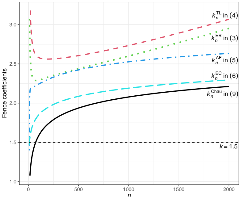
The central object is the fence coefficient $k_n^{\mathrm{Chau}}=\Phi^{-1}(1-0.25/n)/1.35-0.5$, a sample-size-dependent multiplier for the interquartile range in the standard boxplot fences. It does the work by converting Chauvenet's boundary $c_n=\Phi^{-1}(1-0.25/n)$ into an IQR multiplier through the normal-data relations $Q_3-Q_1\approx 1.35 S$ and $(Q_1+Q_3)/2\approx \bar{X}$. A single coefficient then controls whisker length: below Tukey's 1.5 for $n<72$, equal at $n=72$, and growing with $n$ afterward, matching the per-observation false-outside rate that Chauvenet's criterion targets.
What would settle it
Simulate standard normal samples of sizes $n=20,72,500,5000$ many times, and count how many genuine observations fall outside $Q_1-k_n IQR$ and $Q_3+k_n IQR$. The paper's exact-control claim predicts an average of 0.5 flagged observations per sample at every $n$; observed averages differing from 0.5 by more than simulation error, particularly at small $n$, would refute it.
Extended reading notes
Core claim
For normal data, the paper defines new fences $LF_n=Q_1-k_n\times IQR$ and $UF_n=Q_3+k_n\times IQR$ with $k_n=\Phi^{-1}(1-0.25/n)/1.35-0.5$, obtained by equating the boxplot fences to Chauvenet's thresholds $\bar{X}\pm c_n S$ under the normal identities $IQR\approx 1.35 S$ and $(Q_1+Q_3)/2\approx \bar{X}$. It claims this coefficient gives an exact control of the outside rate per observation, that the resulting outlier region is asymptotically equivalent to Chauvenet's criterion, and that because the fences are built on quartiles rather than the sample mean and standard deviation, the rule has a 25% breakdown point. The paper also extends the construction to non-normal data by replacing normal quantiles with quantiles from an estimated parametric distribution, giving separate lower and upper fence coefficients for skewed or heavy-tailed data.
Load-bearing premise
The derivation treats the population normal identities $IQR=1.35\sigma$ and $(Q_1+Q_3)/2=\mu$ as if they hold for sample quartiles, so if sample quartiles deviate from those relations, the per-observation outside rate is only approximately controlled.
Editorial extensions
If this is right
- For normal data, the expected number of genuine observations flagged is about 0.5 regardless of sample size, whereas Tukey's fixed 1.5 fences flag roughly 0.7 percent of a large normal sample.
- Because the fences use quartiles rather than the mean and standard deviation, the rule can detect outliers that classical Chauvenet misses when contamination inflates the standard deviation.
- The new fence coefficient equals Tukey's 1.5 when the sample size is 72; below that the whisker is shorter, increasing detection power for small samples, and above that it lengthens to control false flags.
- For non-normal data, replacing normal quantiles with quantiles from an estimated distribution gives separate lower and upper fence coefficients, which reduces false positives for skewed and heavy-tailed data.
- The rule offers a single, sample-size-aware boxplot that can serve in place of both Tukey's boxplot and Chauvenet's criterion.
Reading between the lines
- Beyond the paper: the same substitution of quartile-based location and scale for the mean and standard deviation could produce robust, sample-size-aware versions of any constant sigma-clipping rule, not only Chauvenet's criterion.
- Beyond the paper: the claimed exact outside-rate control is a population-quantile design target; finite samples will show random fluctuation around 0.5 flagged genuine observations because the quartiles are random, so exactness is best read as the rule's intent rather than a per-sample guarantee.
- Beyond the paper: the non-normal extension assumes the parametric family is known; feeding a nonparametric quantile estimate into the same fence formulas would remove that assumption and can be tested on the same simulation designs.
Editorial analysis
A structured set of objections, weighed in public.
Referee Report
Summary. The paper proposes a sample-size-dependent boxplot fence coefficient, k_n^Chau = Phi^{-1}(1 - 0.25/n)/1.35 - 0.5, obtained by equating the boxplot fences to Chauvenet's criterion under normal-population approximations for the quartiles. It claims that this 'Chauvenet-type boxplot' provides an exact control of the outside rate per observation, is asymptotically equivalent to Chauvenet's criterion (Theorem 1), has a 25% breakdown point, and performs well in simulations and in a Hong Kong civil service pay-adjustment example. A non-normal extension using estimated quantile functions is also proposed, and an R package 'ChauBoxplot' is released on CRAN.
Significance. If rigorously supported, the proposal would fill a practical gap: it offers an explicit, simple, sample-size-adjusted, and quartile-based robust boxplot. The formula in Eq. (9) is parameter-free and easy to implement, the accompanying R package is a concrete deliverable, and the paper is clearly written. The main theoretical contribution, however, is currently an asymptotic approximation, not the claimed exact finite-sample control; this distinction is load-bearing and needs to be corrected before the paper can be recommended for publication.
major comments (3)
- [§3.2, Eq. (9); also abstract and §6] The central claim that the coefficient in Eq. (9) 'provides an exact control of the outside rate per observation' is not established. The derivation in Section 3.2 assumes Q1 + Q3 ≈ 2Xbar and Q3 − Q1 ≈ 1.35S, which are normal-population identities (or asymptotic approximations), not equalities that hold for a finite sample. With random Q1 and Q3, the probability that a normal observation falls outside the fences in Eq. (8) is a function of the joint distribution of these sample quartiles and is not exactly 0.25/n per tail. Theorem 1 establishes only that the thresholds are asymptotically equivalent in ratio; it does not imply exact finite-sample control. The same caveat applies to the original Chauvenet interval in Eq. (7), since Xbar and S are estimated from the same data. The abstract, Section 3.2, and Section 6 should replace 'exact control' with a qualified statement about an asymptotic approximation, or a genuine finite-sample result with quantified error should be provided.
- [§4.1] The simulation evidence for normal data is a single run with set.seed(1863) and two fixed contaminating values (5 and 6). It contains no Monte Carlo replication, so the reported counts cannot substantiate the claims of 'extremely well regardless of the sample size' or of exact control of the outside rate. I recommend reporting averages and standard errors over many replications for each n of (i) the number of genuine observations flagged as outliers, (ii) the number of contaminating observations detected, and (iii) the empirical outside rate for uncontaminated normal samples, which would allow a direct check of the claimed 0.25/n per-tail rate.
- [§5.2, Eqs. (12)–(14)] The non-normal extension is also supported only by a single generated data set of size 50,000, and the assertion that the method 'can perfectly do its job' is stronger than the evidence. The coefficients in Eq. (12) are derived by replacing sample quartiles with F̂^{-1}(0.25) and F̂^{-1}(0.75), so the finite-sample outside rate again depends on estimation error in the parameters and quartiles, which is not quantified. In addition, the t-distribution estimator ν̂ = 2S²/(S²−1) is undefined when S² < 1. These limitations should be acknowledged and the claims scaled back accordingly.
minor comments (5)
- [Abstract and §1] Typos: 'standard derivation' should be 'standard deviation'; this error appears in the abstract and in the introduction.
- [§2.3] The expression 'Φ−1(1 − α/2)1/n)' has a misplaced parenthesis; it should be 'Φ−1((1 − α/2)1/n)'.
- [§3.3] 'ploted' should be 'plotted'; in §2.4, 'expect for' should be 'except for'; in §4.2, 'Fore more details' should be 'For more details'.
- [§6] The statement 'kChau_n = 3 when n = 217, 282' is ambiguous; if two sample sizes are intended, they should be written as 'n = 217 and n = 282'.
- [§3.3] The sentence that the fences 'remain unchanged' when fewer than 25% of observations are outliers is imprecise: quartile-based statistics have a positive breakdown point, but they can still move under contamination below that fraction. A precise definition of the finite-sample replacement breakdown point for the fences would be helpful.
Circularity Check
The 'exact outside rate' claim is imported from Chauvenet's threshold by construction; the new boxplot coefficient itself is otherwise a genuine, non-circular derivation.
-
self definitional
[Section 3.2, Eq. (9) and the paragraph immediately following Eq. (9)]
"Now to fuse Tukey's boxplot with Chauvenet's criterion, we apply the upper 0.25/n quantile of the standard normal distribution, i.e. cn = Φ−1(1 − 0.25/n), as the threshold for labeling anomalous observations. This leads to 1.35kn + 0.675 = Φ−1(1 − 0.25/n), or equivalently, kn = Φ−1(1 − 0.25/n)/1.35 − 0.5."
The coefficient k_n^Chau is defined by solving 1.35 k_n + 0.675 = c_n, which is exactly the condition that makes the boxplot fences in (8) algebraically equal to Chauvenet's interval Xbar ± c_n S under the approximations Q1 ≈ Xbar − 0.675 S and Q3 ≈ Xbar + 0.675 S. The subsequent assertion that the Chauvenet-type boxplot 'provides an exact control of the outside rate per observation' is therefore not derived from a finite-sample distributional calculation involving the random quartiles Q1 and Q3; it is simply the Chauvenet threshold c_n, converted into boxplot units by the very equation that defines k_n^Chau. In other words, the claimed exact property is a restatement of the construction's defining equation, not an independent consequence of the new outlier rule.
full rationale
The paper's main construction is not circular in the usual sense: k_n^Chau is a new, explicit function of n, and Theorem 1 is a genuine asymptotic statement about sample quantiles converging to their population counterparts. No load-bearing self-citations are present, and no fitted parameter is relabeled as a prediction. The circularity concern is narrower and specific to the headline claim of 'exact control of the outside rate per observation.' That property is inherited from Chauvenet's criterion through the sample-level identifications Q1 + Q3 ≈ 2 Xbar and Q3 − Q1 ≈ 1.35 S, which are population approximations, not finite-sample distributional facts. Since Eq. (9) is literally the solution to the equation that forces the boxplot fence to equal the Chauvenet threshold, the exact-rate claim reduces to the defining equation under those approximations. The finite-sample error from replacing quartiles with their population limits is never quantified, and the simulation in Section 4.1 is a single-seed illustration rather than a replication study. This makes the central claim overstated, but the derivation of the coefficient itself remains an independent contribution, so the circularity score is moderate rather than high.
Assumptions & free parameters
free parameters (2)
- Normal approximation constant for IQR to sigma ratio =
1.35
- Chauvenet rate constant =
0.25
assumptions (2)
- domain assumption Sample data are normally distributed for the main construction.
- domain assumption Sample quartiles converge to population quantiles at the rate needed for the approximation.
Cite this review
Pith. "Pith review of When Tukey meets Chauvenet: a new boxplot criterion for outlier detection." pith.science (2026). https://pith.science/paper/DHMEYTOY
@misc{pith2026250606491,
  author       = {Pith},
  title        = {Pith review of: When Tukey meets Chauvenet: a new boxplot criterion for outlier detection},
  year         = {2026},
  howpublished = {\url{https://pith.science/paper/DHMEYTOY}},
  note         = {Machine review of arXiv:2506.06491}
}
read the original abstract
The box-and-whisker plot, introduced by Tukey (1977), is one of the most popular graphical methods in descriptive statistics. On the other hand, however, Tukey's boxplot is free of sample size, yielding the so-called "one-size-fits-all" fences for outlier detection. Although improvements on the sample size adjusted boxplots do exist in the literature, most of them are either not easy to implement or lack justification. As another common rule for outlier detection, Chauvenet's criterion uses the sample mean and standard derivation to perform the test, but it is often sensitive to the included outliers and hence is not robust. In this paper, by combining Tukey's boxplot and Chauvenet's criterion, we introduce a new boxplot, namely the Chauvenet-type boxplot, with the fence coefficient determined by an exact control of the outside rate per observation. Our new outlier criterion not only maintains the simplicity of the boxplot from a practical perspective, but also serves as a robust Chauvenet's criterion. Simulation study and a real data analysis on the civil service pay adjustment in Hong Kong demonstrate that the Chauvenet-type boxplot performs extremely well regardless of the sample size, and can therefore be highly recommended for practical use to replace both Tukey's boxplot and Chauvenet's criterion. Lastly, to increase the visibility of the work, a user-friendly R package named `ChauBoxplot' has also been officially released on CRAN.
Figures

Figures from the paper (3 more)


Reference graph
Works this paper leans on
-
[1]
Abuzaid, A. H., Mohamed, I. B. and Hussin, A. G. (2012). Boxplot for circular variables, Stat 27: 381–392. Andrews, D. F. (1974). A robust method for multiple linear regression,Technometrics 16: 523–531. Andrews, D. F. and Pregibon, D. (1978). Finding the outliers that matter, Journal of the Royal Statistical Society: Series B 44: 1–36. Atkinson, A. C. (1...
work page 2012
-
[2]
McGill, R., Tukey, J. W. and Larsen, W. A. (1978). Variations of box plots,The American Statisti- cian 32: 12–16. 28 Milton, J. S. (1999). Statistical Methods in the Biological and Health Sciences , New York: WCB/McGraw-Hill. Mirzargar, M., Whitaker, R. T. and Kirby, R. M. (2014). Curve boxplot: generalization of box- plot for ensembles of curves, IEEE Tr...
work page 1978
-
[163]
Peirce, B. (1878). On Peirce’s criterion,Proceedings of the American Academy of Arts and Sciences 13: 348–351. Pukelsheim, F. (1994). The three sigma rule, The American Statistician 48: 88–91. Qu, Z. and Genton, M. G. (2022). Sparse functional boxplots for multivariate curves, Journal of Computational and Graphical Statistics 31: 976–989. Raj, M., Mirzarg...
work page 1994
-
[1501]
Carey, V . J., Walters, E. E., Wager, C. G. and Rosner, B. A. (1997). Resistant and test-based outlier rejection: effect on Gaussian one- and two-sample inference, Technometrics 39: 320–330. Carling, K. (2000). Resistant outlier rules and the non-Gaussian case,Computational Statistics and Data Analysis 33: 249–258. Casella, G. and Berger, R. L. (2002). St...
work page 1997
Reviewed August 7, 2026 · model on record in the stance chip above.
Discussion (0). Sign in to comment.