REVIEW 4 major objections 5 minor 38 references
Learning Neural Controllers with Optimality and Stability Guarantees Using Input-Output Dissipativity
T0 review · 4 major / 5 minor · reviewed 2026-08-07 · deepseek-v4-flash
Pith's one-line read The paper constructs a neural feedback controller $\pi(x) = -R(x)^{-1}S(x)^{\top}x$ and proves, under learned dissipativity certificates, that it asymptotically stabilizes the closed loop and is optimal for an explicitly built…
desk verdict The learning pipeline is useful and the experiments are promising, but the SMT verification as written does not certify the matrix definiteness conditions that the stability and optimality theorems require; the gap is concrete and repairable, and the paper deserves a serious referee after revision. read the letter →
The pith
A machine-rendered reading of the paper's core claim, the machinery that carries it, and where it could break.
The reading
What carries the argument
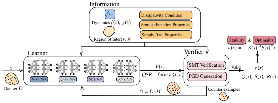
The load-bearing identity is the completion of squares in the dissipation inequality: with $v = u + R(x)^{-1}S(x)^{\top}x$, the supply rate becomes $x^{\top}\Delta(x)x + v^{\top}R(x)v$, and the feedback that zeros $v$ is $\pi = -R^{-1}S^{\top}x$. The matrix $\Delta = S R^{-1} S^{\top} - Q$ measures the excess of the cross and control terms over the state term, and it is the margin that makes $V$ a Lyapunov function. A second ingredient is the matrix inequality (22), whose positive definiteness is equivalent to the $u$-dependent dissipation inequality, reducing the sampling dimension; the same Schur-complement form is what the SMT verifier checks. The cost-shaping loss (29) aligns the constructed running cost with a user-specified objective, so the optimality certificate is with respect to the user's intended performance metric.
What would settle it
Run the verifier on a two-state system with $R(x) = \begin{bmatrix}1&2\\2&1\end{bmatrix}$ and a region contained in a small ball around $(1,1)$. Within that region $x^{\top}R x > 0$ for every $x$, but $R$ is indefinite because it has eigenvalue $-1$ along $(1,-1)$, which lies outside the region, so the paper's scalar check would certify $R(x)\succ0$ even though the positive-definiteness assumption of Theorems 5 and 6 is false. At $x=0$ the same scalar conditions read $0>0$ and are trivially unsatisfiable, so the verification protocol must either exclude the origin or switch to genuine matrix definiteness checks.
Extended reading notes
Core claim
The central result is Theorem 6, stated on the paper's own terms: if $V(x)>0$ and $Q,S,R$ satisfy the dissipation inequality $\partial_x V\,[f(x)+g(x)u] \le x^{\top}Q(x)x + 2x^{\top}S(x)u + u^{\top}R(x)u$ for all $x,u$, with $R(x)>0$ and $\Delta(x)=S(x)R(x)^{-1}S(x)^{\top}-Q(x)>0$, then $\pi(x)=-R(x)^{-1}S(x)^{\top}x$ is the optimal feedback for the infinite-horizon problem with running cost $\tilde{l}(x,u)+u^{\top}R(x)u+x^{\top}\Delta(x)x$, where $\tilde{l}$ captures the residual of the dissipation inequality, and $V(x)$ is the value function. Theorem 5 is the companion stability statement: the same controller gives closed-loop decrease $\dot{V}(x) \le -x^{\top}\Delta(x)x < 0$. Proposition 8 re-expresses the dissipation inequality as a matrix inequality $M(x)\succ 0$ that depends on $x$ alone, so training and verification sample states instead of state-input pairs. Under extra equalities, Proposition 7 reduces the optimality cost to $u^{\top}R(x)u + x^{\top}\Delta(x)x$.
Load-bearing premise
The load-bearing premise is that verifying the scalar inequalities $x^{\top}\Delta(x)x > 0$ and $x^{\top}R(x)x > 0$ over the state region certifies the matrix positive-definiteness conditions $\Delta(x)\succ0$ and $R(x)\succ0$ required by Theorems 5 and 6, an equivalence that fails when the region does not contain all state directions, when the system has multiple inputs, or at $x=0$.
Editorial extensions
If this is right
- A trained and verified tuple $(V,Q,S,R)$ yields a controller with an explicit Lyapunov function $V$ on the verified region, so stability is certified rather than inferred from rollouts.
- The same controller is optimal for a cost the paper explicitly constructs, and Proposition 7 identifies conditions under which that cost is exactly $u^{\top}R(x)u + x^{\top}\Delta(x)x$.
- Cost shaping (29) lets the designer steer the constructed running cost toward a user-defined $l(x,u)$, making the optimality guarantee meaningful for a chosen objective.
- Because the certificate is input-output based, the resulting controller stabilizes any system sharing the same dissipativity property, not only the nominal training dynamics.
- The framework extends to dynamic controllers through an augmented state, which the paper shows generalizes nonlinear PI control.
Reading between the lines
- Beyond the paper: the optimality theorem is inverse optimality — it constructs a cost for which the stabilizing feedback is optimal; it does not say the learned controller is optimal for an arbitrary user cost, only that the shaped cost approximates it, and the paper does not quantify the suboptimality gap when those differ.
- Beyond the paper: the scalar verification shortcuts in Section 4.2 are safe only for scalar-input systems and state regions that contain all state directions; for multi-input plants the theorems require checking matrix positive definiteness, so the framework would need a semidefinite-capable verifier or a parameterization that guarantees $R(x)\succ0$ and $\Delta(x)\succ0$ by construction.
- Beyond the paper: treating $V$ simultaneously as a storage function and a value function suggests a natural way to certify suboptimality — the residual between the learned cost and the true user cost is measurable and could be quoted as a certificate or used to drive further training.
Editorial analysis
A structured set of objections, weighed in public.
Referee Report
Summary. The manuscript proposes a framework for learning neural-network storage functions V(x) and QSR supply-rate functions (Q(x),S(x),R(x)) such that a nonlinear control-affine system satisfies an input-output dissipativity inequality; the controller π(x) = -R(x)^{-1} S(x)^T x is then claimed to asymptotically stabilize the closed loop and to be optimal for an infinite-horizon cost constructed from the learned functions. A counterexample-guided training loop with PGD candidate generation and SMT verification is used to certify the required inequalities, and numerical experiments on an electric circuit, an inverted pendulum, and a rod-on-cart compare the resulting controllers against NCLF and trajectory-based optimal control baselines.
Significance. The central idea of learning dissipativity certificates to obtain simultaneously stabilizing and inverse-optimal neural controllers is attractive and timely, and the state-only reformulation of the dissipativity condition (Proposition 8) is a useful dimensionality reduction for sampling. The stability result (Theorem 5) and the inverse-optimality result (Theorem 6) are self-contained and, modulo presentation issues, the underlying algebra is standard and plausible. The paper also ships reproducible code and compares against reasonable baselines. However, the formal verification step in Section 4.2 does not certify the matrix definiteness hypotheses of the theorems, which undermines the claimed stability and optimality guarantees as stated.
major comments (4)
- [Section 4.2, Eqs. (31)-(32)] The reduction of Δ(x)≻0 and R(x)≻0 to the scalar inequalities x^T Δ(x)x > 0 and x^T R(x)x > 0 for all x in X is not a valid certificate. First, R(x) is m×m while x is n-dimensional, so x^T R(x)x is undefined unless n=m; in the paper's own experiments n≠m (pendulum n=2,m=1; rod-on-cart n=4,m=1). Second, even in the square case, at x=0 the inequality reads 0>0 and is false, so the stated condition cannot hold on any set X containing the origin; if X\{0} is intended, the condition only tests the state directions, not arbitrary control directions, and cannot certify strict positive definiteness of R at the origin, which is needed to define R(x)^{-1} and to make the completion-of-squares argument in Theorem 6 valid. Consequently, the SMT certificate as described does not imply the antecedents of Theorems 5 and 6, and the formal guarantees claimed in Sections 3 and 5 are not established.
- [Theorem 6 proof] The proof contains an unjustified separation: it writes J = - min_u ∫ Vdot dt + min_v ∫ v^T R v dt, suggesting that the two minimizations can be performed independently. In fact ∫ Vdot over [0,∞) equals V(x(∞)) - V(x(0)) = -V(x(0)) for every admissible trajectory with lim x(t)=0, so it is a constant independent of u and the separation can be made rigorous; as written, however, the displayed equality is not justified. The same line also replaces u^T R(x)u in the cost integrand (18) with x^T R(x)x, a typo that obscures the argument. These issues are repairable, but the proof as printed is not fully correct.
- [Section 3.2, Eq. (18); Section 4.1, Eq. (29)] The optimality guarantee is inverse-optimal by construction: Theorem 6 certifies π as optimal for the cost l̃ + u^T R u + x^T Δ x, which is written in terms of the learned functions V,Q,S,R. The user-defined cost l(x,u) enters only through the soft least-squares shaping loss (29), and Theorem 6 gives no bound on the suboptimality of π with respect to that user cost. The abstract's phrase 'inheriting optimality properties that can be shaped towards user-defined control objectives' should be qualified accordingly; the experimental match to LQR on the circuit is encouraging but is not a certificate.
- [Theorem 5 statement] The theorem statement says '0 ≺ R(x) : X → R^{n×n}', but R(x) should map to R^{m×m} since u ∈ R^m in the supply rate (6). This is not merely cosmetic: the dimensional mismatch in Eq. (32) is partly caused by conflating the state dimension n with the input dimension m, and correcting the statement makes it clear that the scalar verification cannot cover the required matrix inequality.
minor comments (5)
- [Theorem 6 proof] The expression 'min_v ∫ v^T R(x)vdt' near the end of the proof is missing the 'dt' inside the integrand; it should read 'min_v ∫ v^T R(x)v dt'.
- [Table 1] The 'Region of interest' entries are ambiguous: 'Pendulum Static [π, 2]' presumably denotes [-π,π]×[-2,2], and 'RodCart [0.1, 0.1, 0.1, 0.1]' presumably denotes [-0.1,0.1]^4; please state the intended boxes explicitly.
- [After Theorem 5] The paragraph on necessity refers to 'the dissipativity matrix condition (22)' before Eq. (22) is introduced in Proposition 8; reorder these two parts or add a forward reference.
- [Section 4.2] The phrase 'equivalent and verifiable algebraic constraints' is misleading for (31)-(32) given the issues raised in the major comments; please use a formulation such as 'relaxations used in verification' and state the exact conditions that the SMT solver checks.
- [Section 4.2] dReal is δ-complete, so the verification results are only correct up to the precision parameter δ (set to 10^{-3} in the experiments); the paper should state clearly that the certificates are approximate in this sense.
Circularity Check
Theorem 6's optimality claim is built from the learned V,Q,S,R by a completion of squares, so the 'optimality guarantee' is true by construction; only the stability result is independently derived.
-
self definitional
[Section 3.2, Theorem 6, Eqs. (18)-(19)]
"Then, π(x) = −R(x)−1S(x)⊤x is the optimal solution of the following optimal control problem with positive definite running cost: min_{u(·)} ∫_0^∞ [˜l(x, u) + u^⊤R(x)u + x^⊤∆(x)x] dt ... where ˜l(x, u) = − ∂V (x)/∂x f (x) − ∂V (x)/∂x g(x)u + x^⊤Q(x)x + 2x^⊤S(x)u. ... Substituting v = u + R(x)−1S(x)⊤x ... since R(x) ≻ 0 ..., the minimum ... is attained at v = 0. From (19), we obtain that the nonlinear control u = −R(x)−1S(x)⊤x is the optimal solution and the storage function V (x) is the optimal value function."
The theorem defines the running cost in terms of the same learned functions that define the controller, and the proof selects v = u + R^{-1}S^T x so that the integrand becomes -dot V + v^T R v. Consequently π is optimal for the constructed cost by construction: minimizing that cost is equivalent to setting the completion-of-squares term to zero, which is exactly the proposed feedback law. The user's cost l enters only through the soft finite-sample square loss Lc in Eq. (29), so Theorem 6 certifies nothing about l; the empirical cost comparisons in Section 5 report the fitted objective rather than a prediction. This makes the optimality half of the paper's central claim self-definitional, while the stability half (Theorem 5) rests on the independent dissipativity inequality.
full rationale
The circularity is limited to the optimality certificate. Theorem 6's cost (18) is assembled from V,Q,S,R and the proof completes the square with v = u + R^{-1}S^T x, so the claimed optimal controller is the minimizer of the constructed cost by construction. This is inverse optimality presented as a guarantee; it is not a derivation of optimality for a pre-specified user cost. The soft shaping loss Lc only fits the constructed cost to the user cost on finitely many samples, so subsequent statements about matching user objectives are not formally supported. The stability argument is not circular: Theorem 5 requires the dissipativity inequality and Δ(x) ≻ 0, and the closed-loop decrease of V follows from the supply rate. The proof's citation of [25] (a co-authored published theorem) is not load-bearing circularity because it is an external, published mathematical result and not a fitted parameter. The verification reduction in Section 4.2, Eqs. (31)-(32), is a correctness gap (scalar conditions cannot certify matrix definiteness when n≠m, and x^T R x is dimensionally ill-posed for R of size m×m), but that is not circularity. Overall, the optimality claim reduces by construction while stability retains independent content, giving a partial circularity score of 6.
Assumptions & free parameters
free parameters (4)
- Neural network weights theta (for V, Q, S, R) =
Not reported
- Bi-Lipschitz constants mu, nu =
Not specified; stated with infeasible ordering 0 < nu < mu
- Loss weights w1..w5 =
Not specified
- SMT precision delta =
10^-3
assumptions (4)
- domain assumption Plant dynamics f, g are known and locally Lipschitz on compact region X
- ad hoc to paper The learned functions satisfy the dissipativity matrix inequality M(x) > 0 on X, as certified by the SMT solver
- ad hoc to paper x^T R(x)x > 0 and x^T Delta(x)x > 0 certify R(x) > 0 and Delta(x) > 0
- standard math lim_{t->inf} x(t) = 0 implies lim_{t->inf} V(x(t)) = 0
Cite this review
Pith. "Pith review of Learning Neural Controllers with Optimality and Stability Guarantees Using Input-Output Dissipativity." pith.science (2026). https://pith.science/paper/5QUK3323
@misc{pith2026250606564,
  author       = {Pith},
  title        = {Pith review of: Learning Neural Controllers with Optimality and Stability Guarantees Using Input-Output Dissipativity},
  year         = {2026},
  howpublished = {\url{https://pith.science/paper/5QUK3323}},
  note         = {Machine review of arXiv:2506.06564}
}
read the original abstract
Deep learning methods have demonstrated significant potential for addressing complex nonlinear control problems. For real-world safety-critical tasks, however, it is crucial to provide formal stability guarantees for the designed controllers. In this paper, we propose a new framework for designing neural controllers that achieve both stability and optimality with respect to certain functions. Our key idea is to exploit the concept of input-output dissipativity of nonlinear systems by learning neural storage functions and supply rate functions. As a generalization of Lyapunov theory, dissipativity theory provides a natural connection to optimal control theory, offering both stability guarantees and meaningful optimality certificates. The neural controllers can be directly derived from the learned supply rate functions and guarantee closed-loop stability while inheriting optimality properties that can be shaped towards user-defined control objectives. Extensive numerical experiments demonstrate the effectiveness of our approach.
Figures


Figures from the paper (1 more)

Reference graph
Works this paper leans on
-
[1]
Deep reinforcement learning for robotics: A survey of real-world successes,
C. Tang, B. Abbatematteo, J. Hu, R. Chandra, R. Mart ´ ın- Mart ´ ın, and P. Stone, “Deep reinforcement learning for robotics: A survey of real-world successes,” Annual Review of Control, Robotics, and Autonomous Systems, vol. 8, 2024
work page 2024
-
[2]
Deep reinforcement learning for intelligent transportation systems: A survey,
A. Haydari and Y. Yılmaz, “Deep reinforcement learning for intelligent transportation systems: A survey,” IEEE Transactions on Intelligent Transportation Systems, vol. 23, no. 1, pp. 11–32, 2020
work page 2020
-
[3]
Review on deep learning applications in frequency analysis and control of modern power system,
Y. Zhang, X. Shi, H. Zhang, Y. Cao, and V. Terzija, “Review on deep learning applications in frequency analysis and control of modern power system,” International Journal of Electrical Power & Energy Systems, vol. 136, p. 107744, 2022
work page 2022
-
[4]
Sastry, Nonlinear systems: analysis, stability, and control , vol
S. Sastry, Nonlinear systems: analysis, stability, and control , vol. 10. Springer Science & Business Media, 2013
work page 2013
-
[5]
Approximate optimal controller synthesis for cart-poles and quadrotors via sums-of-squares,
L. Yang, H. Dai, A. Amice, and R. Tedrake, “Approximate optimal controller synthesis for cart-poles and quadrotors via sums-of-squares,” IEEE Robotics and Automation Letters , 2023
work page 2023
-
[6]
Convex synthesis and verification of control-lyapunov and barrier functions with input constraints,
H. Dai and F. Permenter, “Convex synthesis and verification of control-lyapunov and barrier functions with input constraints,” in 2023 American Control Conference (ACC) , pp. 4116–4123, IEEE, 2023
work page 2023
-
[7]
Advances in computational lyapunov analysis using sum-of-squares programming.,
J. Anderson and A. Papachristodoulou, “Advances in computational lyapunov analysis using sum-of-squares programming.,” Discrete & Continuous Dynamical Systems- Series B , vol. 20, no. 8, 2015
work page 2015
-
[8]
On the construction of lyapunov functions using the sum of squares decomposition,
A. Papachristodoulou and S. Prajna, “On the construction of lyapunov functions using the sum of squares decomposition,” in Proceedings of the 41st IEEE Conference on Decision and Control, 2002., vol. 3, pp. 3482–3487, IEEE, 2002
work page 2002
Show all 38 references
-
[9]
A globally asymptotically stable polynomial vector field with rational coefficients and no local polynomial lyapunov function,
A. A. Ahmadi and B. El Khadir, “A globally asymptotically stable polynomial vector field with rational coefficients and no local polynomial lyapunov function,” Systems & Control Letters, vol. 121, pp. 50–53, 2018
2018
-
[10]
Neural lyapunov control of unknown nonlinear systems with stability guarantees,
R. Zhou, T. Quartz, H. De Sterck, and J. Liu, “Neural lyapunov control of unknown nonlinear systems with stability guarantees,” Advances in Neural Information Processing Systems, vol. 35, pp. 29113–29125, 2022
2022
-
[11]
Neural lyapunov control,
Y.-C. Chang, N. Roohi, and S. Gao, “Neural lyapunov control,” Advances in neural information processing systems, vol. 32, 2019
2019
-
[12]
Learning lyapunov functions for piecewise affine systems with neural network controllers,
S. Chen, M. Fazlyab, M. Morari, G. J. Pappas, and V. M. Preciado, “Learning lyapunov functions for piecewise affine systems with neural network controllers,” arXiv preprint arXiv:2008.06546, 2020
2008 arXiv
-
[13]
Lyapunov-stable neural-network control,
H. Dai, B. Landry, L. Yang, M. Pavone, and R. Tedrake, “Lyapunov-stable neural-network control,” arXiv preprint arXiv:2109.14152, 2021
2021 arXiv
-
[14]
Lyapunov-stable neural control for state and output feedback: A novel formulation,
L. Yang, H. Dai, Z. Shi, C.-J. Hsieh, R. Tedrake, and H. Zhang, “Lyapunov-stable neural control for state and output feedback: A novel formulation,” in Forty-first International Conference on Machine Learning , 2024
2024
-
[15]
Neural lyapunov control for discrete-time systems,
J. Wu, A. Clark, Y. Kantaros, and Y. Vorobeychik, “Neural lyapunov control for discrete-time systems,” Advances in neural information processing systems , vol. 36, pp. 2939– 2955, 2023
2023
-
[16]
Counterexample guided inductive synthesis modulo theories,
A. Abate, C. David, P. Kesseli, D. Kroening, and E. Polgreen, “Counterexample guided inductive synthesis modulo theories,” in International Conference on Computer Aided Verification, pp. 270–288, Springer, 2018
2018
-
[17]
dreal: An smt solver for nonlinear theories over the reals,
S. Gao, S. Kong, and E. M. Clarke, “dreal: An smt solver for nonlinear theories over the reals,” inInternational conference on automated deduction , pp. 208–214, Springer, 2013
2013
-
[18]
Beta-crown: Efficient bound propagation with per-neuron split constraints for neural network robustness verification,
S. Wang, H. Zhang, K. Xu, X. Lin, S. Jana, C.-J. Hsieh, and J. Z. Kolter, “Beta-crown: Efficient bound propagation with per-neuron split constraints for neural network robustness verification,” Advances in Neural Information Processing Systems, vol. 34, pp. 29909–29921, 2021. 11
2021
-
[19]
Evaluating robustness of neural networks with mixed integer programming,
V. Tjeng, K. Xiao, and R. Tedrake, “Evaluating robustness of neural networks with mixed integer programming,” arXiv preprint arXiv:1711.07356, 2017
2017 arXiv
-
[20]
Safety verification and robustness analysis of neural networks via quadratic constraints and semidefinite programming,
M. Fazlyab, M. Morari, and G. J. Pappas, “Safety verification and robustness analysis of neural networks via quadratic constraints and semidefinite programming,” IEEE Transactions on Automatic Control, vol. 67, no. 1, pp. 1–15, 2020
2020
-
[21]
Dissipative dynamical systems part i: General theory,
J. C. Willems, “Dissipative dynamical systems part i: General theory,” Archive for rational mechanics and analysis, vol. 45, no. 5, pp. 321–351, 1972
1972
-
[22]
Nonlinear regulator theory and an inverse optimal control problem,
P. Moylan and B. Anderson, “Nonlinear regulator theory and an inverse optimal control problem,” IEEE Transactions on Automatic Control, vol. 18, no. 5, pp. 460–465, 1973
1973
-
[23]
Dissipativity and optimal control: Examining the turnpike phenomenon,
L. Gr¨ une, “Dissipativity and optimal control: Examining the turnpike phenomenon,” IEEE Control Systems Magazine , vol. 42, no. 2, pp. 74–87, 2022
2022
-
[24]
Nonlinear optimal control for stochastic dynamical systems,
M. Lanchares and W. M. Haddad, “Nonlinear optimal control for stochastic dynamical systems,” Mathematics, vol. 12, no. 5, p. 647, 2024
2024
-
[25]
Necessary and sufficient dissipativity- based conditions for feedback stabilization,
D. d. S. Madeira, “Necessary and sufficient dissipativity- based conditions for feedback stabilization,” IEEE Transactions on Automatic Control, vol. 67, no. 4, pp. 2100– 2107, 2022
2022
-
[26]
Compositional analysis of interconnected systems using delta dissipativity,
K. S. Schweidel and M. Arcak, “Compositional analysis of interconnected systems using delta dissipativity,” IEEE Control Systems Letters , vol. 6, pp. 662–667, 2021
2021
-
[27]
Structured neural- pi control with end-to-end stability and output tracking guarantees,
W. Cui, Y. Jiang, B. Zhang, and Y. Shi, “Structured neural- pi control with end-to-end stability and output tracking guarantees,” Advances in Neural Information Processing Systems, vol. 36, 2024
2024
-
[28]
Synthesizing neural network controllers with closed-loop dissipativity guarantees,
N. Junnarkar, M. Arcak, and P. Seiler, “Synthesizing neural network controllers with closed-loop dissipativity guarantees,” arXiv preprint arXiv:2404.07373 , 2024
2024 arXiv
-
[29]
Learning dissipative neural dynamical systems,
Y. Xu and S. Sivaranjani, “Learning dissipative neural dynamical systems,” IEEE Control Systems Letters , vol. 7, pp. 3531–3536, 2023
2023
-
[30]
Learning chaotic dynamics in dissipative systems,
Z. Li, M. Liu-Schiaffini, N. Kovachki, K. Azizzadenesheli, B. Liu, K. Bhattacharya, A. Stuart, and A. Anandkumar, “Learning chaotic dynamics in dissipative systems,” Advances in Neural Information Processing Systems, vol. 35, pp. 16768–16781, 2022
2022
-
[31]
Learning deep dissipative dynamics,
Y. Okamoto and R. Kojima, “Learning deep dissipative dynamics,” arXiv preprint arXiv:2408.11479 , 2024
2024 arXiv
-
[32]
Sepulchre, M
R. Sepulchre, M. Jankovic, and P. V. Kokotovic,Constructive nonlinear control. Springer Science & Business Media, 2012
2012
-
[33]
Convex optimization,
S. Boyd, “Convex optimization,” Cambridge UP , 2004
2004
-
[34]
Towards deep learning models resistant to adversarial attacks,
A. Madry, “Towards deep learning models resistant to adversarial attacks,” arXiv preprint arXiv:1706.06083, 2017
2017 arXiv
-
[35]
Direct parameterization of lipschitz-bounded deep networks,
R. Wang and I. Manchester, “Direct parameterization of lipschitz-bounded deep networks,” in International Conference on Machine Learning, pp. 36093–36110, PMLR, 2023
2023
-
[36]
Visioli, Practical PID control
A. Visioli, Practical PID control. Springer Science & Business Media, 2006
2006
-
[37]
Equilibrium-independent dissipativity with quadratic supply rates,
J. W. Simpson-Porco, “Equilibrium-independent dissipativity with quadratic supply rates,” IEEE Transactions on Automatic Control, vol. 64, no. 4, pp. 1440–1455, 2018
2018
-
[38]
Global stabilization of polynomial systems using equilibrium-independent dissipativity,
D. d. S. Madeira and T. A. Lima, “Global stabilization of polynomial systems using equilibrium-independent dissipativity,” in 2022 American Control Conference (ACC), pp. 120–125, IEEE, 2022. A Dynamic Control Design Dynamic control is widely used in control theory. One example...
2022
Reviewed August 7, 2026 · model on record in the stance chip above.
Discussion (0). Sign in to comment.