REVIEW 3 major objections 5 minor 50 references
Tensor Stochastic Regression for High-dimensional Time Series via CP Decomposition
T0 review · 3 major / 5 minor · reviewed 2026-08-07 · deepseek-v4-flash
Pith's one-line read A CP low-rank coefficient tensor makes tensor time-series regression tractable at sample size proportional to the sum of mode dimensions.
desk verdict A genuinely new CP tensor stochastic regression framework with real theoretical content, but the exact-rank assumption and the theorem's sample complexity are load-bearing, and the paper's own empirical studies operate outside that regime. read the letter →
The pith
A machine-rendered reading of the paper's core claim, the machinery that carries it, and where it could break.
The reading
What carries the argument
The central object is the CP decomposition $B = \sum_{r=1}^R \omega_r \beta_{r,1} \circ \cdots \circ \beta_{r,N}$, where the unit-norm loading vectors $\beta_{r,d}$ live on the individual modes of the response and predictor tensors and the weights $\omega_r$ set the importance of each rank-one factor. This representation reduces the parameter count from $p_y q_x$ to $R(1 + \sum_d p_d + \sum_d q_d)$ and creates supervised factor processes $f_{r,t} = X_t \times_{d=1}^n \beta_{r,m+d}$ that summarize the predictor tensor. Estimation is carried out by an alternating minimization algorithm adapted from sparse CP tensor regression, with closed-form rank-one updates in the response loadings and ordinary least squares updates in the predictor loadings, optionally followed by hard thresholding for sparsity. The theoretical proof relies on a martingale concentration bound for the dependent design, Hanson-Wright concentration for the linear process $X_t$, restricted strong convexity of the quadratic loss, and covering-number arguments for CP-rank and $\ell_0$-ball parameter sets.
What would settle it
Simulate the model with $B^* = B_{\text{rank }R} + \delta B_{\text{dense}}$, where $\delta B_{\text{dense}}$ is a full-rank perturbation of norm $\delta$, and fit the rank-$R$ estimator for increasing $T$; the claimed rate predicts an error floor proportional to $\delta$, so a clear plateau well above that floor would falsify the exact-rank assumption.
Extended reading notes
Core claim
The paper claims that the tensor stochastic regression model $Y_t = \langle B, X_t\rangle + E_t$, with $Y_t$ an $m$-th order tensor and $X_t$ an $n$-th order tensor, becomes feasible and interpretable when $B$ is assumed to admit the CP decomposition $B = \sum_{r=1}^R \omega_r \beta_{r,1} \circ \cdots \circ \beta_{r,N}$. Under exact CP rank $R$, uniqueness up to permutation, a stationary linear process for the predictors, and sub-Gaussian innovations, the CP low-rank least-squares estimator satisfies $\|\hat B - B^*\|_F = O_p(\sqrt{(\sum_{d=1}^m p_d + \sum_{d=1}^n q_d)\log N / T})$ and a matching prediction-error bound of $O_p((\sum_{d=1}^m p_d + \sum_{d=1}^n q_d)\log N / T)$. When each loading vector is also entrywise sparse with total support $s = \prod_d s_d$, the sparse CP estimator attains $O_p(\sqrt{s\log(p_y q_x)/T})$ for estimation and $O_p(s\log(p_y q_x)/T)$ for prediction. These rates hold for tensor autoregressions as a special case, with the stationarity condition expressed through the spectral radius of the companion matrix.
Load-bearing premise
The guarantees rest on the true coefficient tensor having an exact CP decomposition of known rank $R$ that is unique up to permutation; if the true tensor is only approximately low-rank or the chosen $R$ is wrong, the stated error rates need not hold.
Editorial extensions
If this is right
- When the rank $R$ and the mode dimensions are fixed, the sample size needed for consistent estimation scales with the sum of the mode dimensions rather than the full tensor size $p_y q_x$.
- The framework includes vector, matrix, and tensor autoregressions as special cases, so the paper effectively introduces a CP-based tensor autoregressive model of general lag order with an explicit stationarity condition.
- The sparse CP estimator has an error rate governed by the total support size $s$ rather than the full dimensions, and it can beat Tucker-based estimators when the true factor loadings are sparse.
- Mixed-frequency regression becomes a structured form of unrestricted MIDAS: the loading on the high-frequency mode is estimated from data rather than fixed by a prespecified lag polynomial.
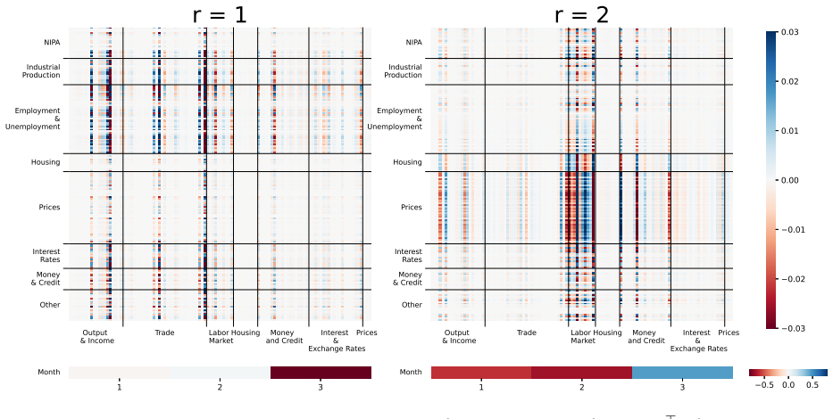
- Pairwise outer products of loading vectors give interpretable maps of response-response, predictor-predictor, and response-predictor interactions, which the paper demonstrates on macroeconomic and air-pollution data.
Reading between the lines
- The theory assumes the true rank $R$ is known and exact; in practice $R$ is selected by cross-validation, so a consistent rank-selection procedure would close the gap between the idealized rates and applied use.
- When the true tensor is only approximately CP low-rank, the estimator should still recover the best rank-$R$ approximation, but the stated exact-rate guarantees would need a bias term proportional to the approximation error.
- The same supervised-factor interpretation could be extended to nowcasting with ragged-edge data, since the high-frequency-mode loading indicates which recent observations matter most for the low-frequency target.
- A direct test of the interpretability claim would be to check whether the learned temporal-aggregation weight $\beta_{r,3}$ matches known publication-lag patterns in macroeconomic data; a mismatch would suggest the model is capturing a different predictive mechanism.
Editorial analysis
A structured set of objections, weighed in public.
Referee Report
Summary. The paper proposes a unified tensor stochastic regression framework, Y_t = <B, X_t> + E_t, with the coefficient tensor B assumed to admit a CP decomposition of rank R. The framework covers vector, matrix, and tensor responses and predictors, and includes tensor autoregression as a special case. Two estimators are studied: a CP low-rank least-squares estimator and a sparse CP low-rank estimator with entrywise ℓ0 constraints on the CP factors. The main theoretical results are non-asymptotic Frobenius-norm estimation and prediction error bounds (Theorems 1 and 2) and analogous bounds for tensor autoregressions (Corollaries 1 and 2). The paper also proposes an alternating minimization algorithm, reports simulation evidence, and applies the methods to mixed-frequency macroeconomic data and Taiwan air pollution data, emphasizing interpretable mode-pair interaction patterns.
Significance. If the stated bounds are correct, the paper provides a broad and useful framework: the CP structure gives parsimonious parametrization and interpretable interactions between modes, and the sparse variant offers additional dimension reduction. The supplement contains detailed proofs using standard tools — restricted strong convexity, Hanson-Wright inequalities for linear processes, martingale concentration, and covering-number arguments — which I found largely plausible. The simulations and the comparisons against Tucker-based and vectorized benchmarks are informative and support the computational and interpretive claims. The main caveats are that the theorems require oracle knowledge of the rank and sparsity levels, that the proofs apply to global minimizers over nonconvex sets while the algorithm lacks convergence guarantees, and that the empirical applications operate far outside the sample-size regime assumed by the theorems.
major comments (3)
- [Section 3.1, Assumption 1, and Supplement Eq. (S5)] The proof of Theorem 1 starts from inequality (S5), loss(B_hat) ≤ loss(B*), which is valid only if the true tensor B* belongs to the feasible set Γ(R) used in the estimator. This requires the practitioner's rank R to be at least the true CP rank. Assumption 1 postulates an exact CP decomposition with R components, but in the methodology the rank is selected by time-series cross-validation (Section 5.1 and Remark S3), and Section 6 explicitly leaves consistent rank selection to future work. If cross-validation selects R smaller than the true rank, B* is infeasible, inequality (S5) fails, and the stated estimation and prediction rates in Theorems 1 and 2 have no support. The same issue applies to the sparsity levels s_d in Assumption 4, which are also selected by cross-validation without a misspecification theory. Please either prove bounds under rank/sparsity misspecification, or state clearly and prominently that the theoretical results are oracle-type and conditional on correct tuning.
- [Sections 5.1 and 5.2] The empirical applications do not satisfy the sample-size condition of the theorems. In the macroeconomic application, T=220, R=40, and ∑_d p_d + ∑_d q_d = 179+112+3 = 294, so the theorem's condition T ≳ (κ2/κ1)^2 R(∑ p_d + ∑ q_d) log N requires at least 40×294×log(3) ≈ 12,900 observations even when (κ2/κ1)^2 = 1. In the air pollution application, T=13, R=4, and the six-mode tensor has ∑ p_d + ∑ q_d = 62, requiring at least 4×62×log(6) ≈ 444 observations under the same optimistic normalization. The empirical sections should not be presented as confirming the theoretical rates; at most they are exploratory illustrations of the method. The authors should add an explicit disclaimer that these applications lie outside the proven validity regime.
- [Section S2, Algorithm 1, and Section 6] Theorems 1 and 2 concern global minimizers of nonconvex optimization problems over CP-rank and sparsity constraint sets, but the estimator actually computed in simulations and applications is the output of Algorithm 1, an alternating minimization procedure. The paper does not establish that the algorithm converges to a global minimizer, and Section 6 states that convergence analysis is left for future work. Consequently, there is a gap between the object for which rates are proven and the object delivered by the implementation. The authors should either provide conditions under which the algorithm's limit satisfies the theorem (for example, initialization guarantees or a risk bound for local optima), or state that the theorems apply only to the global estimator and that the simulation results verify that global estimator, not the algorithm output.
minor comments (5)
- [Section 3.1] There is a typo: "coveriance matrix" should be "covariance matrix".
- [Theorem 1] The probability exponent is printed as 2R(∑_{d=1}^N p_d + 1) log{6(N+1)}; this is ambiguous and should be written as 2R ∑_{d=1}^N (p_d + 1) log{6(N+1)}, with p_{m+d} = q_d.
- [Remark 4] The phrase "strictly stationarity" should be "strictly stationary", and the reference "L·utkepohl" has a formatting artifact.
- [Section 5.2 versus Supplement S4.2] The main text selects R=4 for the sparse estimator, while the supplement's non-sparse CP estimator is later reported as having R=11. The relationship between these two choices should be clarified.
- [Assumption 1] The uniqueness part of Assumption 1, based on the Kruskal-rank condition, is not invoked in the proofs of Theorems 1 and 2, which concern the tensor B_hat rather than its factors. If the assumption is retained for interpretability of the loading vectors, the text should say so explicitly.
Circularity Check
No circularity: the CP-regression rates follow from explicit feasibility and concentration assumptions; self-citations enter only as standard generic lemmas.
full rationale
The derivation chain is not circular. The estimation and prediction error bounds in Theorems 1 and 2 (main text Sections 3.1-3.2; proofs in Supplement S5.3) are obtained by a standard M-estimation argument. The pivotal inequality (S5), used also as (S16) for the sparse case, only requires that both the estimator and the true tensor lie in the same feasible CP-rank or sparsity class; Assumptions 1 and 4 explicitly impose this feasibility (exact rank R and sparsity levels s_d). This is a modelling assumption, not a fitted quantity that is later reported as the theorem's conclusion. The rates are derived by controlling the empirical process with covering-number estimates (Lemmas S.5 and S.6) and with concentration inequalities for linear processes (Lemmas S.1 and S.3) and martingales (Lemma S.4). Some of these lemmas are cited from prior work by the corresponding author (Zheng 2025; Huang et al. 2024), but they are generic spectral, Hanson-Wright, and martingale bounds whose stated assumptions do not contain the tensor-regression error bound; they are standard probabilistic tools, so this is not load-bearing self-citation in the circularity sense. The empirical claims are out-of-sample rolling forecasts on held-out periods (Section S4.1: Q1-2022 through Q4-2022; Section S4.2: year 2017), not in-sample fitted constants relabeled as predictions. The paper itself flags the main limitations in Section 6: rank and sparsity parameters are selected by time-series cross-validation without a consistency theory, and the alternating-minimization algorithm's convergence is not established. A further validity gap, but not a circularity, is that in the macroeconomic application T=220, R=40, and sum_d p_d + sum_d q_d = 294, so the theorem's stated sample-size condition T >= C R (sum_d p_d + sum_d q_d) log N is not satisfied; the empirical results therefore lie outside the theorem's formal regime. None of these considerations make the theoretical derivation equivalent to its inputs.
Assumptions & free parameters
free parameters (2)
- CP rank R =
R=40 for macro data, R=4 for air pollution data (selected by cross-validation)
- Sparsity levels s_d =
s=(4,3,3,4,4,12) for air pollution data
assumptions (5)
- domain assumption Assumption 1: B* has a unique CP decomposition of rank R up to permutation (Kruskal-rank condition).
- domain assumption Assumption 2: Innovations are sub-Gaussian with independent coordinates and are martingale differences with respect to the predictor filtration.
- domain assumption Assumption 3: The predictor process is stationary, has an infinite-order moving average representation with summable coefficients, and the innovation process is sub-Gaussian with dimension q_epsilon <= q_x.
- domain assumption Assumption 4: The true loading vectors are sparse with ||beta*_{r,d}||_0 <= s_d.
- standard math Background results: Hanson-Wright inequality for stationary time series (Lemma S.3), martingale concentration (Lemma S.4), covering number bounds (Lemmas S.5, S.6), and the spectral bounds of the linear process (Lemma S.1).
Cite this review
Pith. "Pith review of Tensor Stochastic Regression for High-dimensional Time Series via CP Decomposition." pith.science (2026). https://pith.science/paper/F3IM4VBL
@misc{pith2026250606919,
  author       = {Pith},
  title        = {Pith review of: Tensor Stochastic Regression for High-dimensional Time Series via CP Decomposition},
  year         = {2026},
  howpublished = {\url{https://pith.science/paper/F3IM4VBL}},
  note         = {Machine review of arXiv:2506.06919}
}
read the original abstract
As tensor-valued data become increasingly common in time series analysis, there is a growing need for flexible and interpretable models that can handle high-dimensional predictors and responses across multiple modes. We propose a unified framework for high-dimensional tensor stochastic regression based on CANDECOMP/PARAFAC (CP) decomposition, which encompasses vector, matrix, and tensor responses and predictors as special cases. Tensor autoregression naturally arises as a special case within this framework. By leveraging CP decomposition, the proposed models interpret the interactive roles of any two distinct tensor modes, enabling dynamic modeling of input-output mechanisms. We develop both CP low-rank and sparse CP low-rank estimators, establish their non-asymptotic error bounds, and propose an efficient alternating minimization algorithm for estimation. Simulation studies confirm the theoretical properties and demonstrate the computational advantage. Applications to mixed-frequency macroeconomic data and spatio-temporal air pollution data reveal interpretable low-dimensional structures and meaningful dynamic dependencies.
Figures


Figures from the paper (2 more)

Reference graph
Works this paper leans on
-
[1]
Babii, A., Ghysels, E., and Pan, J. (2024). Tensor PCA for factor models. Available at SSRN 4791809
work page 2024
-
[2]
Babii, A., Ghysels, E., and Striaukas, J. (2022). Machine Learning Time Series Regressions With an Application to Nowcasting . Journal of Business and Economic Statistics , 40:1094--1106
work page 2022
-
[3]
Bai, J. and Wang, P. (2016). Econometric analysis of large factor models. Annual Review of Economics , 8:53--80
work page 2016
-
[4]
Barigozzi, M., He, Y., Li, L., and Trapani, L. (2022). Statistical inference for large-dimensional tensor factor model by iterative projections. arXiv preprint arXiv:2206.09800
work page Pith review arXiv 2022
-
[5]
Basu, S. and Michailidis, G. (2015). Regularized estimation in sparse high-dimensional time series models. The Annals of Statistics , 43:1535--1567
work page 2015
-
[6]
Bi, X., Tang, X., Yuan, Y., Zhang, Y., and Qu, A. (2021). Tensors in statistics. Annual Review of Statistics and Its Application , 8:345--368
work page 2021
-
[7]
Chan, J. C. C. and Qi, Y. (2024). Large bayesian tensor vars with stochastic volatility. arXiv preprint arXiv:2409.16132
work page Pith review arXiv 2024
-
[8]
Chang, J., He, J., Yang, L., and Yao, Q. (2023). Modelling matrix time series via a tensor cp-decomposition. Journal of the Royal Statistical Society Series B: Statistical Methodology , 85:127--148
work page 2023
Show all 50 references
-
[9]
Chen, B., Han, Y., and Yu, Q. (2024). Estimation and inference for CP tensor factor models. arXiv preprint arXiv:2406.17278
2024
-
[10]
Chen, R., Xiao, H., and Yang, D. (2021a). Autoregressive models for matrix-valued time series. Journal of Econometrics , 222:539--560
2021
-
[11]
Chen, R., Yang, D., and Zhang, C.-H. (2022). Factor models for high-dimensional tensor time series. Journal of the American Statistical Association , 117:94--116
2022
-
[12]
and Lam, C
Chen, W. and Lam, C. (2024). Rank and factor loadings estimation in time series tensor factor model by pre-averaging. The Annals of Statistics , 52:364--391
2024
-
[13]
Chen, Y.-L., Kolar, M., and Tsay, R. S. (2021b). Tensor canonical correlation analysis with convergence and statistical guarantees. Journal of Computational and Graphical Statistics , 30:728--744. Data available at https://github.com/youlinchen/TCCA
2021
-
[14]
Feng, L., Bi, X., and Zhang, H. (2021). Brain regions identified as being associated with verbal reasoning through the use of imaging regression via internal variation. Journal of the American Statistical Association , 116(533):144--158
2021
-
[15]
Foroni, C., Marcellino, M., and Schumacher, C. (2015). Unrestricted mixed data sampling (midas): Midas regressions with unrestricted lag polynomials. Journal of the Royal Statistical Society. Series A (Statistics in Society) , 178:57--82
2015
-
[16]
and Marcellino, M
Foroni, C. and Marcellino, M. G. (2013). A survey of econometric methods for mixed-frequency data. Available at SSRN 2268912
2013
-
[17]
Ghysels, E., Sinko, A., and Valkanov, R. (2006). MIDAS regressions: Further results and new directions. Econometric Reviews , 26:53--90
2006
-
[18]
Han, Y., Yang, D., Zhang, C.-H., and Chen, R. (2024). CP factor model for dynamic tensors . Journal of the Royal Statistical Society Series B: Statistical Methodology , 86:1383–1413
2024
-
[19]
Huang, F., Lu, K., Zheng, Y., and Li, G. (2025). Supervised factor modeling for high-dimensional linear time series. Journal of Econometrics , 249:105995
2025
-
[20]
Kolda, T. G. and Bader, B. W. (2009). Tensor decompositions and applications. SIAM Review , 51:455--500
2009
-
[21]
Kruskal, J. B. (1976). More factors than subjects, tests and treatments: an indeterminacy theorem for canonical decomposition and individual differences scaling. Psychometrika , 41:281--293
1976
-
[22]
Liu, J., Zhu, C., Long, Z., and Liu, Y. (2021). Tensor regression. Foundations and Trends® in Machine Learning , 14:379--565
2021
-
[23]
Lock, E. F. (2018). Tensor-on-tensor regression. Journal of Computational and Graphical Statistics , 27:638--647
2018
-
[24]
and Zhang, A
Luo, Y. and Zhang, A. R. (2024). Tensor-on-tensor regression: Riemannian optimization, over-parameterization, statistical-computational gap, and their interplay. Annals of Statistics . to appear
2024
-
[25]
L\" u tkepohl, H. (2005). New Introduction to Multiple Time Series Analysis . Springer Science & Business Media
2005
-
[26]
McCracken, M. W. and Ng, S. (2016). FRED-MD : A monthly database for macroeconomic research. Journal of Business & Economic Statistics , 34:574--589
2016
-
[27]
McCracken, M. W. and Ng, S. (2021). FRED-QD: A quarterly database for macroeconomic research . Federal Reserve Bank of St. Louis Review , 103:1--44
2021
-
[28]
Raskutti, G., Yuan, M., and Chen, H. (2019). Convex regularization for high-dimensional multi-response tensor regression. Annals of Statistics , 47:1554--1584
2019
-
[29]
Rogers, M., Li, L., and Russell, S. J. (2013). Multilinear dynamical systems for tensor time series. Advances in Neural Information Processing Systems , 26
2013
-
[30]
Samadi, S. Y. and Billard, L. (2024). On a matrix-valued autoregressive model. Journal of Time Series Analysis . to appear
2024
-
[31]
Sidiropoulos, N. D. and Bro, R. (2000). On the uniqueness of multilinear decomposition of n-way arrays. Journal of Chemometrics , 14:229--239
2000
-
[32]
Sun, W. W. and Li, L. (2017). STORE: Sparse tensor response regression and neuroimaging analysis . Journal of Machine Learning Research , 18:1--37
2017
-
[33]
Ten Berge, J. M. and Sidiropoulos, N. D. (2002). On uniqueness in CANDECOMP/PARAFAC . Psychometrika , 67:399--409
2002
-
[34]
Tsay, R. S. (2024). Matrix-variate time series analysis: A brief review and some new developments. International Statistical Review , 92:246--262
2024
-
[35]
P., Reinsel, G
Velu, R. P., Reinsel, G. C., and Wichern, D. W. (1986). Reduced rank models for multiple time series. Biometrika , 73:105--118
1986
-
[36]
Wang, D., Liu, X., and Chen, R. (2019). Factor models for matrix-valued high-dimensional time series. Journal of Econometrics , 208:231--248
2019
-
[37]
Wang, D., Zheng, Y., and Li, G. (2024). High-dimensional low-rank tensor autoregressive time series modeling. Journal of Econometrics , 238(1):105544
2024
-
[38]
Wang, D., Zheng, Y., Lian, H., and Li, G. (2022). High-dimensional vector autoregressive time series modeling via tensor decomposition. Journal of the American Statistical Association , 117(539):1338--1356
2022
-
[39]
Wang, X., Zhu, H., and Initiative, A. D. N. (2017). Generalized scalar-on-image regression models via total variation. Journal of the American Statistical Association , 112(519):1156--1168
2017
-
[40]
and Ng, M
Zeng, C. and Ng, M. K. (2021). Incremental CP tensor decomposition by alternating minimization method. SIAM Journal on Matrix Analysis and Applications , 42:832--858
2021
-
[41]
Zheng, Y. (2025). An interpretable and efficient infinite-order vector autoregressive model for high-dimensional time series. Journal of the American Statistical Association , 120:212--225
2025
-
[42]
Zhou, H., Li, L., and Zhu, H. (2013). Tensor regression with applications in neuroimaging data analysis. Journal of the American Statistical Association , 108(502):540--552
2013
-
[43]
and Teboulle, M
Beck, A. and Teboulle, M. (2009). Iterative shrinkage and thresholding for linear inverse problems. SIAM Journal on Imaging Sciences , 2(1):183--202
2009
-
[44]
M., and Chen, Y
Chi, Y., Lu, Y. M., and Chen, Y. (2019). Nonconvex optimization meets low-rank matrix factorization: An overview. IEEE Transactions on Signal Processing , 67:5239--5269
2019
-
[45]
De Lathauwer, L., De Moor, B., and Vandewalle, J. (2000). A multilinear singular value decomposition. SIAM journal on Matrix Analysis and Applications , 21(4):1253--1278
2000
-
[46]
Huang, F., Lu, K., and Zheng, Y. (2024). SARMA: S calable low-rank high-dimensional autoregressive moving averages via tensor decomposition. ArXiv preprint arXiv:2405.00626
2024 arXiv
-
[47]
J., and Yu, B
Raskutti, G., Wainwright, M. J., and Yu, B. (2011). Minimax rates of estimation for high-dimensional linear regression over _q -balls. IEEE Transactions on Information Theory , 57(10):6976--6994
2011
-
[48]
W., Lu, J., Liu, H., and Cheng, G
Sun, W. W., Lu, J., Liu, H., and Cheng, G. (2017). Provable sparse tensor decomposition. Journal of the Royal Statistical Society Series B: Statistical Methodology , 79(3):899--916
2017
-
[49]
Tibshirani, R. (1996). Regression shrinkage and selection via the lasso. Journal of the Royal Statistical Society: Series B , 58:267–288
1996
-
[50]
Wilms, I., Basu, S., Bien, J., and Matteson, D. (2023). Sparse identification and estimation of large-scale vector autoregressive moving averages. Journal of the American Statistical Association , 118:571–582
2023
Reviewed August 7, 2026 · model on record in the stance chip above.
Discussion (0). Sign in to comment.