REVIEW 4 major objections 5 minor 69 references
Scalable Spatiotemporal Modeling for Bicycle Count Prediction
T0 review · 4 major / 5 minor · reviewed 2026-08-07 · deepseek-v4-flash
Pith's one-line read The paper claims that a Bayesian spatiotemporal dynamic GLM with a random-walking Matérn intercept outperforms Poisson GLM, BKTR, and BayesNF on Montreal bicycle counts, and that its sparse SPDE version is nearly as accurate while 5 to 12…
desk verdict Solid integration of existing Bayesian spatiotemporal machinery with a practical bicycle-count application, but the 'consistently outperforms' claim needs repeated-split evidence before it holds. read the letter →
The pith
A machine-rendered reading of the paper's core claim, the machinery that carries it, and where it could break.
The reading
What carries the argument
The engine is the log-rate decomposition $\lambda_t(s)=\mu_t(s)+F_t'\theta_t+X_t(s)'\beta+\varepsilon_t(s)$, where the spacetime intercept obeys $\mu_t(s)=\mu_{t-1}(s)+\omega_t(s)$ with spatial $\omega_t$ drawn from a Matérn field, and $F_t'\theta_t$ carries harmonics with dynamic coefficients. The sparse counterpart replaces the dense Matérn covariance with the SPDE approximation of Lindgren et al. (2011), writing $\mu_t(s)=a(s)'R_t$ with mesh weights $R_t$ having a sparse Gaussian Markov random field precision matrix; this is what removes the $O(n^3)$ covariance cost. The sampler combines closed-form Gibbs updates for variance parameters, pMALA updates for log-rates, and forward filtering backward sampling for dynamic states.
What would settle it
Compare, at the long-term Eco-counter sites, the empirical variance of daily residuals to their mean: a substantially greater-than-one ratio is direct evidence against the Poisson assumption. Alternatively, hold out the actual partial counts at several short-term sites and check whether the model's AADB posterior intervals cover the directly observed annual totals.
Extended reading notes
Core claim
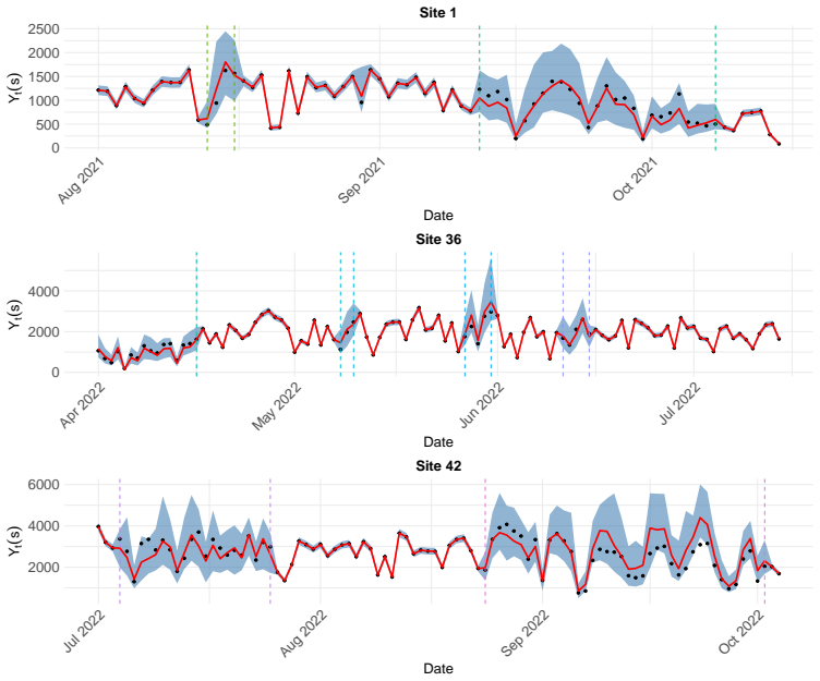
The central claim is that spatiotemporal dependence in bicycle counts can be captured by a Poisson log-rate whose intercept follows a random walk with spatially correlated Matérn innovations, together with dynamically evolving seasonal harmonics and exogenous covariates. The paper develops full Bayesian inference for this model with a hybrid MCMC sampler, then replaces the dense Matérn covariance with the SPDE-based Gaussian Markov random field approximation to make it scale. On the Montreal Island Eco-counter data the dense ST-DGLM produces the lowest MAE, rMSE, and CRPS at all tested missingness levels, the sparse version is competitive and the second best, and both provide natural posterior predictive intervals for imputation, kriging, forecasting, and AADB.
Load-bearing premise
The load-bearing premise is that daily counts at every site are Poisson and that sites with almost no data share the same spatial process and covariate effects as the long-term counters; if either fails, the predicted counts and AADB intervals will be overconfident or biased.
Editorial extensions
If this is right
- Long-term count sites can impute their own missing blocks and obtain posterior predictive intervals, not just point estimates.
- Short-term and brand-new sites can receive AADB estimates and uncertainty without a full year of observed data.
- Forecasts and spatiotemporal predictions at future times and unobserved locations are available from the same fitted model.
- The sparse version makes the model usable when the number of sites or mesh nodes is large, with a tunable accuracy-speed tradeoff through mesh size.
- Planners get an interpretable alternative to ML/DL models, since each component corresponds to a trend, season, weather effect, or site effect.
Reading between the lines
- The paper does not test the Poisson assumption against an overdispersed count model; if daily counts are overdispersed, the reported credible intervals are likely too narrow.
- The 93 short-term sites are treated as completely unobserved, so their few actual counts could validate the AADB interpolation, a check the paper does not run.
- Because the spatial field is Euclidean, the model ignores street-network distance; a graph-based Matérn would be a natural next test and could tighten interpolation along cycling corridors.
- The same hierarchical structure could transfer directly to pedestrian counts or other sensor-based count data with similar seasonality and spatial correlation.
Editorial analysis
A structured set of objections, weighed in public.
Referee Report
Summary. The paper proposes a Bayesian spatiotemporal dynamic generalized linear model (ST-DGLM) for daily bicycle counts. The log-rate is modeled as the sum of a space-time varying intercept that evolves as a random walk with Matérn spatial innovations, purely temporal dynamic coefficients driven by a state-space evolution, fixed covariate effects, and i.i.d. normal nuggets. A sparse version replaces the dense Matérn field with the SPDE/GMRF approximation of Lindgren et al. (2011). Inference is carried out with a custom hybrid MCMC sampler combining Gibbs updates, FFBS for the dynamic coefficients, and pMALA for the Poisson log-rates. The model is evaluated on synthetic data and on Montreal Eco-counter bicycle counts, where it is compared with a Poisson GLM, BKTR, and BayesNF, and is used to impute missing values, krige unobserved sites, and estimate average annual daily bicycles (AADB). The paper claims that ST-DGLM consistently outperforms the alternatives while maintaining interpretability and uncertainty quantification.
Significance. If the predictive claims hold, the framework would provide a useful interpretable and uncertainty-aware tool for bicycle-count imputation, kriging, forecasting, and AADB estimation, and the SPDE extension is a sensible route to scalability. The paper ships a substantial methodological contribution: a customized hybrid MCMC sampler, explicit predictive machinery for several target quantities, and an implementation in an R package. The synthetic experiment demonstrates the feasibility of the sampler and the accuracy of the sparse approximation for data generated from the same model hierarchy. However, the external evidence for the central 'consistently outperforms' claim rests on a single real-data holdout configuration and on comparisons against baselines that use a different response family, so the strength of the empirical conclusions currently exceeds what the evaluation supports.
major comments (4)
- [Section 5.3, Table 3] The real-data evidence for the central claim that ST-DGLM 'consistently outperforms alternatives' (Section 6) is based on a single holdout configuration: four sites removed entirely and four additional sites with three missingness masks. The three rows in Table 3 are not independent replications; they are the same held-out sites evaluated under different missing-data patterns. No site-level replication, repeated random splits, cross-validation, or uncertainty in the reported MAE/rMSE/CRPS values is provided, so the large margins over BKTR and BayesNF could reflect the particular choice of held-out sites rather than systematic superiority. This is load-bearing because the real-data benchmark is the primary external validation of the framework. I recommend either adding repeated site-holdout or k-fold evaluation with error bars and paired comparisons, or substantially tempering the 'consistently outperforms' claim.
- [Section 5.2, Section 5.3, Table 3] The comparison with BKTR and BayesNF is confounded by response family: BKTR is fit to log-transformed counts under a normal response, and BayesNF uses a normal observation model on log-transformed counts, while ST-DGLM is a Poisson count model. Differences in MAE/rMSE/CRPS may therefore reflect the likelihood family rather than the spatiotemporal modeling contribution. The paper should either adapt BKTR and BayesNF to count-compatible observation models (e.g., Poisson or negative binomial likelihoods), or explicitly justify and discuss the comparability of log-normal approximations on the count scale, including how predictive draws are transformed before computing CRPS.
- [Section 3.3, Section 5.3, Eq. (13)] A key claimed contribution is AADB estimation at short-term and unobserved sites, but the 93 short-term sites with partial data are treated as completely unobserved and no validation of the AADB predictions against the available partial counts is reported. Because these sites sometimes have one or two days of actual counts, a direct check of whether the predicted AADB is consistent with those observations would substantially strengthen the AADB claim. As written, the AADB results in Figure 5 are not externally grounded.
- [Section 2.1, Eq. (1)] The conditional Poisson assumption is not checked against overdispersion or other count-data misspecification. Although the normal nugget term induces a Poisson-log-normal marginal distribution, the paper does not perform posterior predictive checks, dispersion diagnostics, or a comparison with an overdispersed alternative. If the conditional Poisson assumption is violated, the reported CRPS values and credible intervals, including those used for AADB uncertainty, may be overconfident. A concrete test, such as a posterior predictive check based on the observed count variances or a negative binomial extension, would address this concern.
minor comments (5)
- [Section 1.1] There are several typos in the introduction, including 'severeal', 'colunts', and 'Toaddressthesechallenges'; these should be corrected.
- [Section 4, Table 1] Table 1 uses 'rMSPE' in the caption while the text and main results use 'rMSE'; the notation should be unified. Also, the sentence 'we gain in computational efficiency but lose in efficiency' should say 'lose in accuracy'.
- [Section 5.2] The covariate description contains a stray 'w.' at the end of a sentence, and 'censors' should be 'sensors'. The covariate names in Table 4 (e.g., βws(s)) should be matched consistently with the text referring to 'bβwalk'.
- [Section 4, Appendix C] Because the synthetic data are generated from the model hierarchy in Eq. (C1), the recovery of intercepts and coefficients is a self-consistency result that validates the MCMC implementation and mesh approximation, but it should not be presented as external validation of the model. The paper largely frames it correctly, but the wording could be made more explicit.
- [Data and Code Availability] The sparseDGLM package is currently only available on request and is planned for public release later. Making the code and a vignette available with the paper would improve reproducibility and allow readers to verify the computational claims.
Circularity Check
No circularity identified: the derivation chain is self-contained, and the real-data predictive claims rest on independent holdout comparisons.
full rationale
I walked the paper's derivation chain and found no step where a prediction or first-principles result reduces, by the paper's own equations or by a load-bearing self-citation, to its own inputs. The synthetic experiment in Section 4 generates data from the model hierarchy in Eq. (C1)/(A1) and then checks whether the true generating parameters and latent states are recovered; this is a standard simulation-based coherence check of the MCMC sampler and of the SPDE approximation, and the paper explicitly frames it that way ('validating both the efficacy of our MCMC sampler ... and the accuracy of the sparse ST-DGLM model'). That self-consistency exercise is not used as evidence for the model's real-world superiority. The central empirical claim that 'the ST-DGLM framework consistently outperforms alternatives' (Section 6) is supported by Table 3, where four sites are removed entirely and four additional sites are masked at 50%, 60%, and 80% missingness, and predictions at these held-out observations are compared against Poisson GLM, BKTR, and BayesNF. This is a genuine out-of-sample comparison, not a fitted parameter renamed as a prediction. The AADB estimates at the 93 short-term sites are spatially interpolated without validation against their partial counts, but that is a limitation in external validation, not a definitional circularity. The self-citations present (Cisneros et al. 2023, Hazra et al. 2024, Lei et al. 2024, Lanthier et al. 2023) are methodological or competitor references and none carries a load-bearing premise such as a uniqueness theorem. The principal weaknesses--a single holdout split without site-level replication, an untested Poisson/overdispersion assumption, and unvalidated AADB interpolation--are statistical support concerns and should be weighed as correctness risk, not as circularity.
Assumptions & free parameters
free parameters (6)
- beta (regression coefficients) =
e.g., temperature 0.286, precipitation -0.361 (Table 4)
- kappa (Matérn range) =
5.08 km (Table 4); 0.356 in synthetic
- sigma^2 (spatial intercept variance) =
0.084 (Table 4)
- tau^2 (nugget variance) =
0.016 (Table 4)
- W (state evolution variances w1..w4) =
0.013, 0.012, 0.019, 0.029 (Table 4)
- nu (Matérn smoothness) =
0.5 in application, 1 in synthetic
assumptions (4)
- domain assumption Conditional Poisson distribution for daily counts at each site given log-rate (Eq. 1)
- domain assumption Random-walk evolution of the space-time intercept with Gaussian Matérn innovations (Eq. 3)
- standard math SPDE approximation with alpha=2 provides a valid discrete approximation to the Matérn field (Eqs. 6-7)
- ad hoc to paper Inverse-gamma priors with shape=2, rate=0.1 for variance parameters
Cite this review
Pith. "Pith review of Scalable Spatiotemporal Modeling for Bicycle Count Prediction." pith.science (2026). https://pith.science/paper/VSH4J6ZO
@misc{pith2026250607582,
  author       = {Pith},
  title        = {Pith review of: Scalable Spatiotemporal Modeling for Bicycle Count Prediction},
  year         = {2026},
  howpublished = {\url{https://pith.science/paper/VSH4J6ZO}},
  note         = {Machine review of arXiv:2506.07582}
}
read the original abstract
We propose a novel sparse spatiotemporal dynamic generalized linear model for efficient inference and prediction of bicycle count data. Assuming Poisson distributed counts with spacetime-varying rates, we model the log-rate using spatiotemporal intercepts, dynamic temporal covariates, and site-specific effects additively. Spatiotemporal dependence is modeled using a spacetime-varying intercept that evolves smoothly over time with spatially correlated errors, and coefficients of some temporal covariates including seasonal harmonics also evolve dynamically over time. Inference is performed following the Bayesian paradigm, and uncertainty quantification is naturally accounted for when predicting bicycle counts for unobserved locations and future times of interest. To address the challenges of high-dimensional inference of spatiotemporal data in a Bayesian setting, we develop a customized hybrid Markov Chain Monte Carlo (MCMC) algorithm. To address the computational burden of dense covariance matrices, we extend our framework to high-dimensional spatial settings using the sparse SPDE approach of Lindgren et al. (2011), demonstrating its accuracy and scalability on both synthetic data and Montreal Island bicycle datasets. The proposed approach naturally provides missing value imputations, kriging, future forecasting, spatiotemporal predictions, and inference of model components. Moreover, it provides ways to predict average annual daily bicycles (AADB), a key metric often sought when designing bicycle networks.
Figures


Figures from the paper (2 more)

Reference graph
Works this paper leans on
-
[1]
, " * write output.state after.block = add.period write newline
ENTRY address author booktitle chapter edition editor howpublished institution isbn journal key month note number organization pages publisher school series title type volume year label extra.label sort.label short.list INTEGERS output.state before.all mid.sentence after.sentence after.block FUNCTION init.state.consts #0 'before.all := #1 'mid.sentence :=...
-
[2]
write newline
" write newline "" before.all 'output.state := FUNCTION n.dashify 't := "" t empty not t #1 #1 substring "-" = t #1 #2 substring "--" = not "--" * t #2 global.max substring 't := t #1 #1 substring "-" = "-" * t #2 global.max substring 't := while if t #1 #1 substring * t #2 global.max substring 't := if while FUNCTION word.in bbl.in capitalize " " * FUNCT...
-
[3]
Ahmadi, S. A., Ghasemi, P. and Ehmke, J. F. (2024) Optimizing urban bike-sharing systems: a stochastic mathematical model for infrastructure planning. Central European Journal of Operations Research pp. 1--35
work page 2024
-
[4]
Albuquerque, V., Sales Dias, M. and Bacao, F. (2021) Machine learning approaches to bike-sharing systems: A systematic literature review. ISPRS International Journal of Geo-Information 10(2), 62
work page 2021
-
[5]
Almannaa, M. H., Elhenawy, M. and Rakha, H. A. (2020) Dynamic linear models to predict bike availability in a bike sharing system. International journal of sustainable transportation 14(3), 232--242
work page 2020
- [6]
-
[7]
Bakka, H., Rue, H., Fuglstad, G.-A., Riebler, A., Bolin, D., Illian, J., Krainski, E., Simpson, D. and Lindgren, F. (2018) Spatial modeling with R-INLA : A review. Wiley Interdisciplinary Reviews: Computational Statistics 10(6), e1443
work page 2018
-
[8]
Banerjee, S., Carlin, B. P. and Gelfand, A. E. (2014) Hierarchical M odeling and A nalysis for S patial D ata . Second edition. CRC Press
work page 2014
Show all 69 references
-
[9]
and Miranda-Moreno, L
Beitel, D., McNee, S. and Miranda-Moreno, L. F. (2017) Quality measure of short-duration bicycle counts. Transportation Research Record 2644(1), 64--71
2017
-
[10]
and Kooperberg, C
Besag, J. and Kooperberg, C. (1995) On conditional and intrinsic autoregressions. Biometrika 82(4), 733--746
1995
-
[11]
and Durrande, N
Borovitskiy, V., Azangulov, I., Terenin, A., Mostowsky, P., Deisenroth, M. and Durrande, N. (2021) Mat \'e rn G aussian processes on graphs. In International Conference on Artificial Intelligence and Statistics, pp. 2593--2601
2021
-
[12]
and Prozzi, J
Buddhavarapu, P., Bansal, P. and Prozzi, J. A. (2021) A new spatial count data model with time-varying parameters. Transportation Research Part B: Methodological 150, 566--586
2021
-
[13]
Carter, C. K. and Kohn, R. (1994) On G ibbs sampling for state space models. Biometrika 81(3), 541--553
1994
-
[14]
Chen, J., Li, K., Li, K., Yu, P. S. and Zeng, Z. (2021) Dynamic planning of bicycle stations in dockless public bicycle-sharing system using gated graph neural network. ACM Transactions on Intelligent Systems and Technology (TIST) 12(2), 1--22
2021
-
[15]
and Huser, R
Cisneros, D., Gong, Y., Yadav, R., Hazra, A. and Huser, R. (2023) A combined statistical and machine learning approach for spatial prediction of extreme wildfire frequencies and sizes. Extremes 26(2), 301--330
2023
-
[16]
and Tsapakis, I
Das, S. and Tsapakis, I. (2020) Interpretable machine learning approach in estimating traffic volume on low-volume roadways. International Journal of Transportation Science and Technology 9(1), 76--88
2020
-
[17]
Datta, A., Banerjee, S., Finley, A. O. and Gelfand, A. E. (2016) Hierarchical nearest-neighbor G aussian process models for large geostatistical datasets. Journal of the American Statistical Association 111(514), 800--812
2016
-
[18]
and Yu, Z
Duan, Y., Zhang, S. and Yu, Z. (2021) Applying B ayesian spatio-temporal models to demand analysis of shared bicycle. Physica A: Statistical Mechanics and its Applications 583, 126296
2021
-
[19]
A., Reich, B
Eidsvik, J., Shaby, B. A., Reich, B. J., Wheeler, M. and Niemi, J. (2014) Estimation and prediction in spatial models with block composite likelihoods. Journal of Computational and Graphical Statistics 23(2), 295--315
2014
-
[20]
and Uz, V
Eren, E. and Uz, V. E. (2020) A review on bike-sharing: The factors affecting bike-sharing demand. Sustainable cities and society 54, 101882
2020
-
[21]
and Hadden Loh, T
Ermagun, A., Lindsey, G. and Hadden Loh, T. (2018) Bicycle, pedestrian, and mixed-mode trail traffic: a performance assessment of demand models. Landscape and Urban Planning 177, 92--102
2018
-
[22]
and Zhou, Y
Feng, J., Liu, H., Zhou, J. and Zhou, Y. (2024) A spatial-temporal aggregated graph neural network for docked bike-sharing demand forecasting. ACM Transactions on Knowledge Discovery from Data 18(9), 1--27
2024
-
[23]
(2016) Bikeshare: A review of recent literature
Fishman, E. (2016) Bikeshare: A review of recent literature. Transport reviews 36(1), 92--113
2016
-
[24]
and Calderhead, B
Girolami, M. and Calderhead, B. (2011) Riemann manifold L angevin and hamiltonian M onte C arlo methods. Journal of the Royal Statistical Society Series B: Statistical Methodology 73(2), 123--214
2011
-
[25]
and Raftery, A
Gneiting, T. and Raftery, A. E. (2007) Strictly proper scoring rules, prediction, and estimation. Journal of the American statistical Association 102(477), 359--378
2007
-
[26]
Y., Dauwels, J., Mitrovic, N., Asif, M
Goh, C. Y., Dauwels, J., Mitrovic, N., Asif, M. T., Oran, A. and Jaillet, P. (2012) Online map-matching based on hidden M arkov model for real-time traffic sensing applications. In 2012 15th International IEEE Conference on Intelligent Transportation Systems, pp. 776--781
2012
-
[27]
Guidon, S., Reck, D. J. and Axhausen, K. (2020) Expanding a (n)(electric) bicycle-sharing system to a new city: Prediction of demand with spatial regression and random forests. Journal of Transport Geography 84, 102692
2020
-
[28]
and Gneiting, T
Guttorp, P. and Gneiting, T. (2006) Studies in the history of probability and statistics XLIX on the M at \'e rn correlation family. Biometrika 93(4), 989--995
2006
-
[29]
and Sun, Y
Hazra, A., Nag, P., Yadav, R. and Sun, Y. (2024) Exploring the efficacy of statistical and deep learning methods for large spatial datasets: A case study. Journal of Agricultural, Biological and Environmental Statistics pp. 1--24
2024
-
[30]
J., Datta, A., Finley, A
Heaton, M. J., Datta, A., Finley, A. O., Furrer, R., Guinness, J., Guhaniyogi, R., Gerber, F., Gramacy, R. B., Hammerling, D., Katzfuss, M. et al. (2019) A case study competition among methods for analyzing large spatial data. Journal of Agricultural, Biological and Environmen...
2019
-
[31]
H., Bardin, E
Hochmair, H. H., Bardin, E. and Ahmouda, A. (2019) Estimating bicycle trip volume for M iami- D ade county from S trava tracking data. Journal of Transport Geography 75, 58--69
2019
-
[32]
(2016) Estimation of annual average daily traffic (AADT) and missing hourly volume using artificial intelligence
Islam, S. (2016) Estimation of annual average daily traffic (AADT) and missing hourly volume using artificial intelligence. Master's thesis, Clemson University
2016
-
[33]
K., Klein, N
Kaiser, S. K., Klein, N. and Kaack, L. H. (2025) From counting stations to city-wide estimates: data-driven bicycle volume extrapolation. Environmental Data Science 4, e13
2025
-
[34]
and Guinness, J
Katzfuss, M. and Guinness, J. (2021) A general framework for V ecchia approximations of G aussian processes
2021
-
[35]
and Rue, H
Krainski, E., G \'o mez-Rubio, V., Bakka, H., Lenzi, A., Castro-Camilo, D., Simpson, D., Lindgren, F. and Rue, H. (2018) Advanced spatial modeling with stochastic partial differential equations using R and INLA. Chapman and Hall/CRC
2018
-
[36]
and Labbe, A
Lanthier, J., Lei, M., Sun, L. and Labbe, A. (2023) BKTR : An efficient spatiotemporally varying coefficient regression package in R and P ython
2023
-
[37]
and Nakamura, Y
Lee, D., Kulic, D. and Nakamura, Y. (2008) Missing motion data recovery using factorial hidden M arkov models. In 2008 IEEE International Conference on Robotics and Automation, pp. 1722--1728
2008
-
[38]
and Sun, L
Lei, M., Labbe, A. and Sun, L. (2024) Scalable spatiotemporally varying coefficient modeling with B ayesian kernelized tensor regression. Bayesian Analysis 1(1), 1--29
2024
-
[39]
and Sun, L
Lei, M., Labbe, A., Wu, Y. and Sun, L. (2022) Bayesian kernelized matrix factorization for spatiotemporal traffic data imputation and kriging. IEEE Transactions on Intelligent Transportation Systems 23(10), 18962--18974
2022
-
[40]
and Rue, H
Lindgren, F. and Rue, H. (2015) Bayesian spatial modelling with R-INLA . Journal of statistical software 63, 1--25
2015
-
[41]
and Lindstr \"o m, J
Lindgren, F., Rue, H. and Lindstr \"o m, J. (2011) An explicit link between G aussian fields and G aussian M arkov random fields: the stochastic partial differential equation approach. Journal of the Royal Statistical Society: Series B (Statistical Methodology) 73(4), 423--498
2011
-
[42]
and Jonsson, D
Liu, C., Tapani, A., Kristoffersson, I., Rydergren, C. and Jonsson, D. (2020) Development of a large-scale transport model with focus on cycling. Transportation research part a: Policy and practice 134, 164--183
2020
-
[43]
M., Hyun, K
Miah, M. M., Hyun, K. K., Mattingly, S. P. and Khan, H. (2023) Estimation of daily bicycle traffic using machine and deep learning techniques. Transportation 50(5), 1631--1684
2023
-
[44]
(2023) Open data
Montréal, B. (2023) Open data. https://bixi.com/en/open-data. Accessed: 2023-07-11
2023
-
[45]
E., Janson, B
Nordback, K., Marshall, W. E., Janson, B. N. and Stolz, E. (2013) Estimating annual average daily bicyclists: Error and accuracy. Transportation research record 2339(1), 90--97
2013
-
[46]
and Campagnoli, P
Petris, G., Petrone, S. and Campagnoli, P. (2009) Dynamic linear models with R. Springer Science & Business Media
2009
-
[47]
and Yanchenko, A
Pherwani, P., Hass, N. and Yanchenko, A. K. (2024) Spatiotemporal modeling and forecasting at scale with dynamic generalized linear models. arXiv preprint arXiv:2410.07161
2024 arXiv
-
[48]
and Soyer, R
Ravishanker, N., Raman, B. and Soyer, R. (2022) Dynamic Time Series Models Using R-INLA: An Applied Perspective. Chapman and Hall/CRC
2022
-
[49]
(2015) Bike sharing: A review of evidence on impacts and processes of implementation and operation
Ricci, M. (2015) Bike sharing: A review of evidence on impacts and processes of implementation and operation. Research in Transportation Business & Management 15, 28--38
2015
-
[50]
Roberts, G. O. and Rosenthal, J. S. (2009) Examples of adaptive MCMC . Journal of computational and graphical statistics 18(2), 349--367
2009
-
[51]
and Held, L
Rue, H. and Held, L. (2005) Gaussian Markov random fields: theory and applications. CRC press
2005
-
[52]
and Chopin, N
Rue, H., Martino, S. and Chopin, N. (2009) Approximate B ayesian inference for latent G aussian models by using integrated nested L aplace approximations. Journal of the Royal Statistical Society Series B: Statistical Methodology 71(2), 319--392
2009
-
[53]
Ruiz-C \'a rdenas, R., Krainski, E. T. and Rue, H. (2012) Direct fitting of dynamic models using integrated nested L aplace approximations— INLA . Computational Statistics & Data Analysis 56(6), 1808--1828
2012
-
[54]
Saurous, R
Saad, F., Burnim, J., Carroll, C., Patton, B., K \"o ster, U., A. Saurous, R. and Hoffman, M. (2024) Scalable spatiotemporal prediction with B ayesian neural fields. Nature Communications 15(1), 7942
2024
-
[55]
Schmidt, A. M. and Lopes, H. F. (2019) Dynamic models. In Handbook of environmental and ecological statistics, pp. 57--80. Chapman and Hall/CRC
2019
-
[56]
and Sadabadi, K
Sekula, P., Markovic, N., Vander Laan, Z. and Sadabadi, K. F. (2018) Estimating historical hourly traffic volumes via machine learning and vehicle probe data: A maryland case study. Transportation Research Part C: Emerging Technologies 97, 147--158
2018
-
[57]
and Winters, M
Sersli, S., Gislason, M., Scott, N. and Winters, M. (2022) Easy as riding a bike? bicycling competence as (re) learning to negotiate space. Qualitative research in sport, exercise and health 14(2), 268--288
2022
-
[58]
and Shibasaki, R
Song, X., Kanasugi, H. and Shibasaki, R. (2016) Deeptransport: Prediction and simulation of human mobility and transportation mode at a citywide level. In Proceedings of the twenty-fifth international joint conference on artificial intelligence, pp. 2618--2624
2016
-
[59]
Strauss, J., Miranda-Moreno, L. F. and Morency, P. (2013) Cyclist activity and injury risk analysis at signalized intersections: a bayesian modelling approach. Accident Analysis & Prevention 59, 9--17
2013
-
[60]
P., da Silva, A
Teixeira, I. P., da Silva, A. N. R., Schwanen, T., Manzato, G. G., D \"o rrzapf, L., Zeile, P., Dekoninck, L. and Botteldooren, D. (2020) Does cycling infrastructure reduce stress biomarkers in commuting cyclists? a comparison of five european cities. Journal of Transport Geog...
2020
-
[61]
F., Silva, C
Teixeira, J. F., Silva, C. and Moura e S \'a , F. (2021) Empirical evidence on the impacts of bikesharing: a literature review. Transport reviews 41(3), 329--351
2021
-
[62]
Vecchia, A. V. (1988) Estimation and model identification for continuous spatial processes. Journal of the Royal Statistical Society Series B: Statistical Methodology 50(2), 297--312
1988
-
[63]
and Ni, W
Wang, X. and Ni, W. (2016) An improved particle filter and its application to an ins/gps integrated navigation system in a serious noisy scenario. Measurement Science and Technology 27(9), 095005
2016
-
[64]
and Harrison, J
West, M. and Harrison, J. (1997) Bayesian Forecasting and Dynamic Models. Second edition. Springer
1997
-
[65]
West, M., Harrison, P. J. and Migon, H. S. (1985) Dynamic generalized linear models and bayesian forecasting. Journal of the American Statistical Association 80(389), 73--83
1985
-
[66]
(1954) On stationary processes in the plane
Whittle, P. (1954) On stationary processes in the plane. Biometrika pp. 434--449
1954
-
[67]
(2016) Modeling Seasonal and Weather Impacts on Cycling Count
Zhao, W. (2016) Modeling Seasonal and Weather Impacts on Cycling Count. Ph.D. thesis
2016
-
[68]
and Yang, K
Zhou, C., Hu, J., Zhang, X., Li, Z. and Yang, K. (2024) A bike-sharing demand prediction model based on spatio-temporal graph convolutional networks. PeerJ Computer Science 10, e2391
2024
-
[69]
(2015) Understanding spatiotemporal patterns of biking behavior by analyzing massive bike sharing data in C hicago
Zhou, X. (2015) Understanding spatiotemporal patterns of biking behavior by analyzing massive bike sharing data in C hicago. PloS one 10(10), e0137922
2015
Reviewed August 7, 2026 · model on record in the stance chip above.
Discussion (0). Sign in to comment.