REVIEW 4 major objections 5 minor 88 references
An environmental analysis of supernova iPTF13bvn with HST and MUSE
T0 review · 4 major / 5 minor · reviewed 2026-08-07 · deepseek-v4-flash
Pith's one-line read An environmental analysis of supernova iPTF13bvn resolves two stellar populations and points to the older, roughly $20\,M_\odot$ one as its binary-stripped progenitor.
desk verdict A careful, transparent environmental study of iPTF13bvn whose central claim about an older binary progenitor population is real but rests on UV non-detections and a post-hoc population choice; still worth serious referee time. read the letter →
The pith
A machine-rendered reading of the paper's core claim, the machinery that carries it, and where it could break.
The reading
What carries the argument
The central machinery is a hierarchical Bayesian mixture model — a statistical model that treats the 138 resolved stars inside the 300-parsec aperture as drawn from several underlying stellar populations — sampled with nested sampling. Stars missing from a filter enter the analysis as censored detections: their magnitudes are replaced by the 50-percent-recovery detection limit found from artificial-star tests, and the likelihood uses the cumulative normal distribution of that limit. Distance modulus and stellar mass are marginalised away with a Salpeter initial-mass function, the binary fraction is fixed at 0.5, and the number of population components (one to four) is chosen by corrected Bayesian evidence on the Jeffreys scale. On the gas side, the Balmer decrement — the ratio of $H\alpha$ to $H\beta$ flux, converted to extinction with intrinsic ratios for gas temperatures of 2500 to 20000 K — turns each integral-field spaxel into a line-of-sight dust measurement. Resampling the HST images onto the same spaxel grid puts stars, gas, and dust on a common scale, so the two probes can be compared geometrically.
What would settle it
Re-observe the iPTF13bvn site at ultraviolet wavelengths substantially deeper than the existing F225W image, and check whether the stars predicted by the P2 isochrone appear or whether the 93 non-detections were artifacts of an overly optimistic detection-limit model. Alternatively, refit the same photometric catalogue with a different completeness function and test whether the Bayesian evidence still prefers two populations over one, and whether the older population still lands near $20.0\,M_\odot$.
Extended reading notes
Core claim
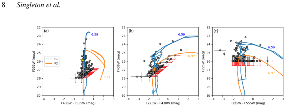
The paper's central claim is that the environment of iPTF13bvn contains two distinct stellar populations — a younger one with $\tau_1 = 6.59^{+0.04}_{-0.05}$ and $A_{V,1} = 0.95^{+0.07}_{-0.06}$ mag, and an older one with $\tau_2 = 6.97^{+0.06}_{-0.06}$ and $A_{V,2} = 0.53^{+0.10}_{-0.08}$ mag, separated by about 5.4 million years of star formation. The older population, P2, is the decisive one: its extinction matches the $A_V \approx 0.53$ mag derived in earlier color-based analyses, the initial mass of its most massive stars ($20.0\,M_\odot$) falls inside the range expected for a binary progenitor, and the absence of any bright H II region near the explosion site favors a longer-lived, lower-mass star over a short-lived very massive one. The paper therefore asserts that iPTF13bvn's hydrogen envelope was stripped predominantly by binary interaction rather than by stellar winds, and that the combination of resolved stellar photometry and ionized-gas spectroscopy can break the single-versus-binary degeneracy that direct progenitor imaging alone has not settled. The mass-loss channel matters beyond this one supernova, because single-star winds cannot by themselves produce the observed rates and diversity of stripped-envelope supernovae.
Load-bearing premise
Everything rests on the older population P2 being real, but P2 is pinned down almost entirely by ultraviolet non-detections: 93 of the 138 environment stars enter the fit as F225W detection limits, and the paper concedes that only a handful of fully detected stars constrain that population, so an inaccurate completeness model could make P2 — and with it the binary-progenitor conclusion — a fitting artifact.
Editorial extensions
If this is right
- If P2 is the natal population, iPTF13bvn's progenitor had a zero-age main-sequence mass near $20.0\,M_\odot$ and must have been stripped by a companion, because single stars of that mass do not lose enough mass through winds to explode as hydrogen-poor supernovae.
- The lack of any bright H II region at the explosion site means the traditional "nearest H II region" shortcut would have overestimated this progenitor's mass; the paper suggests using H II-region association as the diagnostic, favoring the oldest resolved population when no association is found.
- The extinction ladder — P2 at 0.53 mag, P1 at 0.95 mag, ionized gas near 1.7–1.9 mag — yields a three-dimensional line-of-sight arrangement of the stars and dust, extending an interpretation developed for two other supernovae in the same host galaxy.
- Environments on spiral-arm edges show substantially higher extinction variability than smooth arm interiors, so assuming one smooth value for population parameters there — as Voronoi binning or pixel statistics do — can misrepresent the true properties of the progenitor.
- Applied to a catalogue of nearby core-collapse supernovae, the method could assign individual events to single-star versus binary mass-loss channels without requiring a fortuitous pre-explosion image of each star.
Reading between the lines
- The choice of P2 over P1 rests on statistical agreement with prior progenitor studies, not on an independent identification; a surviving-companion search or a kinematic measurement of the environment would give the decisive test the paper does not attempt.
- Because 93 of the 138 stars enter the fit as ultraviolet detection limits, the two-population result is conditional on the completeness model for those non-detections; a deeper ultraviolet observation that recovers the predicted old-population stars directly would be the cleanest confirmation.
- The foreground-stars/background-gas reading of the extinction gap is one consistent geometry, but the data do not exclude dust in front of the stars; independent dust tracers across the same region could test the three-dimensional picture.
- If the pattern holds for other events, Type Ib supernovae on spiral-arm edges without H II-region association should systematically point to lower-mass binary progenitors — a sample-level prediction testable with the growing set of integral-field follow-up observations.
Editorial analysis
A structured set of objections, weighed in public.
Referee Report
Summary. The paper presents an environmental study of the Type Ib supernova iPTF13bvn using HST/WFC3 photometry of resolved stars within a 300 pc region and VLT/MUSE IFU spectroscopy of the ionized gas. A hierarchical Bayesian mixture model with nested sampling is applied to isochrone fitting, yielding two stellar populations: P1 with log-age 6.59 and A_V = 0.95 mag, and P2 with log-age 6.97 and A_V = 0.53 mag. The authors identify P2 as the likely natal population because its age and extinction correspond to an initial mass of about 20 M_sun and an extinction of 0.53 mag, consistent with binary progenitor models from Bersten et al. (2014) and Eldridge et al. (2015). The MUSE analysis finds no bright H II region at the SN site, gas extinctions roughly 2.5 to 3.6 times higher than the stellar population values, and increased extinction variability on the edge of the spiral arm. The paper concludes that the environment supports a binary progenitor for iPTF13bvn.
Significance. If the identification of P2 as the host population is robust, the paper provides a valuable template for combining resolved stellar photometry with IFU gas maps to break degeneracies in supernova progenitor studies, and it would strengthen the case that iPTF13bvn's progenitor was a roughly 20 M_sun star in a binary system. The authors are transparent about limitations, notably that only a handful of stars with complete photometry constrain the older population, and they compare their results quantitatively with previous studies in Table 4. The statistical machinery is standard, the data are public, and the multi-wavelength approach is clearly described. However, the central claim rests on the existence and parameters of P2, which are inferred largely from F225W non-detections, and on a post-hoc assignment of P2 as the natal population; these load-bearing points need additional support before the conclusion can be accepted.
major comments (4)
- [Section 3.1, Figure 2] The evidence for two stellar populations is not quantified. The text states that the largest relative jump in corrected Bayesian evidence is between the N_m = 1 and N_m = 2 models and invokes the Jeffreys scale with a threshold of about 30, but the actual numerical values of ln Z or Delta ln Z are not reported, and the figure subplot does not allow verification. Because the entire P2 analysis depends on this model choice, please report the numerical evidence values for N_m = 1 through 4 and demonstrate that the increase between N_m = 1 and N_m = 2 exceeds the stated threshold. Ideally, add a posterior predictive check or a cross-validation comparison between one- and two-population fits.
- [Section 4.1 and Eq. (3)] The older population P2, on which the 20.0 M_sun binary-progenitor conclusion rests, is constrained dominantly by F225W detection-limit substitutions: 93 of 138 stars use Eq. (3) in F225W, and the text acknowledges that only a handful of stars with complete photometry constrain P2. The sensitivity of tau_P2, A_V,P2, and the resulting mass to the assumed detection limits (m_lim, sigma_lim) and to the completeness model is not tested. Please refit the model with detection limits varied within their quoted uncertainties and with the F225W filter excluded; if P2's parameters shift by more than the quoted 1-sigma errors, or if the two-population evidence drops below the Jeffreys threshold, the central claim would need to be weakened substantially.
- [Section 4.1, Table 4] The assignment of P2 as the host population is post-hoc: P2 is preferred because it matches the Bersten et al. (2014) and Eldridge et al. (2015) progenitor constraints, while the paper itself states that there is no independent check. Figure 4a shows that the progenitor photometry overlaps both isochrones, and the alternative assignment (P1) would imply a much higher initial mass of about 65.4 M_sun. The conclusion that the results support a binary progenitor is therefore not directly entailed by the environmental analysis alone. Either provide an independent diagnostic that selects P2 before comparison with progenitor models, or reframe the conclusion as showing consistency with, rather than direct support for, a binary progenitor.
- [Section 3.1] The conversion from population age to progenitor mass uses the maximum mass on the isochrone as the best estimate. This is an ad-hoc assumption: in a sparse population of 138 stars, the maximum mass is subject to sampling fluctuations, and the progenitor need not be the most massive star present or even near the isochrone turnoff. The quoted M_initial,P2 = 20.0 M_sun should be accompanied by an uncertainty that accounts for IMF sampling and for the range of masses consistent with the fitted age; otherwise the mass estimate is not well defined.
minor comments (5)
- [Section 3.1 vs Section 4.2.3] The extinction dispersion conversion is inconsistent: Section 3.1 defines sigma_AV,k = 0.05 x 10^delta_AV,k, while Section 4.2.3 uses 0.058 x 10^delta_AV,k. Please harmonize the two expressions.
- [Section 3.5] The starburst99 comparison quotes ages without errors and states that the EW errors fall inside the age resolution of the models; please state the model age grid step explicitly so that the reader can assess the granularity of the comparison.
- [Section 2.2.1] The sentence 'Given that (14,14) occurs at the centre of the spaxel, we can confidently conclude that iPTF13bvn falls inside this spaxel' is slightly confusing because the transformed position (14.17, 14.19) is already inside the spaxel; rephrase for clarity.
- [Table 4 and Section 4.2.1] The distance used for 'This Work' is 22.5 Mpc, but the text notes distance estimates extending to 27.4 Mpc and states that a larger distance would increase the progenitor mass. Consider adding a systematic uncertainty to M_initial from the distance modulus, since this directly affects the central mass claim.
- [Figure 4 caption] There is a typo in the caption: 'environmnet' should be 'environment'. Also, the labels 'pop1' and 'pop2' in the figure are informal; consider using 'P1' and 'P2' to match the text.
Circularity Check
Photometric two-population fit is self-contained, but the binary-progenitor conclusion rests on a post-hoc selection of P2 as the host because it matches prior binary constraints, with the paper conceding no independent check.
-
other
[Section 4.1 (Host Resolved Population), Table 4 discussion and following paragraph]
"the progenitor converges on a binary system with a primary initial mass within the range of 10−20 M⊙, ending its life as a low-mass helium star. This aligns with our results for P2: A_V,P2 = 0.53+0.10−0.08 mag; M_initial,P2 = 20.0 M⊙ ... Overall, the results of this paper are able to reproduce the populations found by Maund (2018) and Sun et al. (2023), as well as a new population that agrees with the progenitor constraints for iPTF13bvn from the remaining studies in Table 4."
The paper's binary-progenitor conclusion depends on designating P2 as the natal population. That designation is made because P2's fitted parameters (A_V = 0.53 mag, M_initial = 20.0 M_sun) agree with the same binary-progenitor constraints from Bersten et al. (2014) and Eldridge et al. (2015) that the conclusion then claims to 'support'. The agreement is therefore the selection criterion rather than an independent confirmation. The photometric fit itself never uses those constraints (flat priors; likelihood from photometry only), so this is a post-hoc interpretive loop rather than an equation-level reduction. The paper's own statement, 'we still do not have an independent check', explicitly concedes the limitation.
full rationale
The core derivation is not circular at the equation level. P1 and P2 ages, extinctions, and dispersions are obtained from a hierarchical Bayesian mixture model applied to HST/WFC3 photometry with flat priors on tau and A_V (Section 3.1), and the nested-sampling evidence comparison is performed on the photometry alone. The MUSE Balmer-decrement and EW analyses are likewise independent of the progenitor constraints. Self-citations to Maund & Ramirez-Ruiz (2016), Maund (2018), and Sun et al. (2021, 2023) supply methodology, not the result, and the method is re-implemented with ultranest on new public data, so they are not load-bearing in a circular way. The only circularity-like step is the interpretive assignment of P2 as the host population: P2 is selected because its parameters agree with prior binary-progenitor studies, and the same agreement is then presented as support for a binary progenitor. The paper explicitly acknowledges there is no independent check of this assignment, which limits but does not eliminate the concern. An additional robustness caveat (not circularity) is that P2 is constrained largely by F225W detection-limit substitutions rather than complete photometry, so its parameters may be fragile; this affects confidence in the conclusion but does not make the photometric fit itself circular. Overall score 3 reflects one acknowledged post-hoc interpretive loop while the statistical and spectroscopic derivations remain self-contained.
Assumptions & free parameters
free parameters (7)
- Population 1 age tau1 =
6.59 (+0.04/-0.05) log years
- Population 1 extinction A_V,1 =
0.95 (+0.07/-0.06) mag
- Population 1 extinction dispersion sigma_AV,1 =
0.346 mag
- Population 2 age tau2 =
6.97 (+0.06/-0.06) log years
- Population 2 extinction A_V,2 =
0.53 (+0.10/-0.08) mag
- Population 2 extinction dispersion sigma_AV,2 =
0.097 mag
- Population weights omega_k =
Dirichlet-normalized; one independent weight
assumptions (7)
- standard math The stellar mass prior follows a Salpeter (1955) IMF with exponent -2.35, normalized over the mass range of the PARSEC models.
- domain assumption PARSEC stellar isochrones (Girardi et al. 2002) with fixed solar metallicity Z=0.02 describe the stellar populations.
- ad hoc to paper Binary fraction P_bin = 0.5 in the mixture model, fixed throughout.
- domain assumption Intrinsic Balmer decrement ratios from Osterbrock & Ferland (2006) for electron temperatures 2500 to 20000 K apply to the ionized gas.
- domain assumption Cardelli et al. (1989) extinction law with R_V = 3.1 applies to both foreground and host-galaxy dust.
- ad hoc to paper The maximum mass on the isochrone at the fitted population age approximates the initial mass of the SN progenitor.
- domain assumption Distance to NGC 5806 is 22.5 Mpc (Tully et al. 2009), with distance modulus 31.76+/-0.36 mag.
Cite this review
Pith. "Pith review of An environmental analysis of supernova iPTF13bvn with HST and MUSE." pith.science (2026). https://pith.science/paper/JQMMPMW3
@misc{pith2026250608099,
  author       = {Pith},
  title        = {Pith review of: An environmental analysis of supernova iPTF13bvn with HST and MUSE},
  year         = {2026},
  howpublished = {\url{https://pith.science/paper/JQMMPMW3}},
  note         = {Machine review of arXiv:2506.08099}
}
abstract
Searches for supernovae (SNe) progenitors have relied on a direct detection of the star in fortuitous pre-explosion images. We propose an alternative method, using a combination of photometric stellar population fitting alongside integral-field-unit (IFU) spectroscopic analysis of the ionised gas to fully explore the SN environment and constrain the progenitor properties. Isochrone fitting of HST/WFC3 observations reveals the environment of iPTF13bvn contains two stellar populations with unique age ($\tau=\log{t [years]}$) and extinction ($A_V$) values, with the closest agreement found between past progenitor studies of iPTF13bvn and our oldest stellar population (P2): $\tau_{P2}=6.97^{+0.06}_{-0.06}$, a corresponding initial mass $M_{initial,P2} = 20.0 M_\odot$ and $A_{V,P2}=0.53^{+0.10}_{-0.08}$ mag. Further analysis with VLT/MUSE IFU-spectroscopic observations reveals no bright H II regions associated with iPTF13bvn, suggesting no immediate ongoing star formation. Extinctions derived from the ionised gas are a minimum of ~2.5 times higher than the resolved stellar population values, assisting in building a 3D picture of the environment. An analysis of the distribution of spaxel extinctions reveals increased variability in the environment of iPTF13bvn, on the edge of a spiral arm. Our study highlights the complex relationship between stars, gas and dust and how, when used in a holistic environmental analysis, they can begin to resolve degeneracies that have plagued past progenitor investigations. Specifically for iPTF13bvn, our results support a binary progenitor and a growing consensus for binarity as the predominant mass-loss mechanism for Type Ib SNe progenitors.
Figures


Figures from the paper (4 more)


Reference graph
Works this paper leans on
-
[1]
write newline
" write newline "" before.all 'output.state := FUNCTION fin.entry write newline FUNCTION new.block output.state before.all = 'skip after.block 'output.state := if FUNCTION new.sentence output.state after.block = 'skip output.state before.all = 'skip after.sentence 'output.state := if if FUNCTION not #0 #1 if FUNCTION and 'skip pop #0 if FUNCTION or pop #1...
-
[2]
Aldering G., Humphreys R. M., Richmond M., 1994, @doi [ ] 10.1086/116886 , https://ui.adsabs.harvard.edu/abs/1994AJ....107..662A 107, 662
doi:10.1086/116886 1994
-
[3]
Anderson J. P., James P. A., 2008, @doi [ ] 10.1111/j.1365-2966.2008.13843.x , https://ui.adsabs.harvard.edu/abs/2008MNRAS.390.1527A 390, 1527
arXiv 2008
-
[4]
Anderson J. P., Covarrubias R. A., James P. A., Hamuy M., Habergham S. M., 2010, @doi [ ] 10.1111/j.1365-2966.2010.17118.x , https://ui.adsabs.harvard.edu/abs/2010MNRAS.407.2660A 407, 2660
arXiv 2010
-
[5]
Anderson J. P., James P. A., Habergham S. M., Galbany L., Kuncarayakti H., 2015, @doi [ ] 10.1017/pasa.2015.19 , https://ui.adsabs.harvard.edu/abs/2015PASA...32...19A 32, e019
-
[6]
Aryan A., et al., 2021, @doi [ ] 10.1093/mnras/stab1379 , https://ui.adsabs.harvard.edu/abs/2021MNRAS.505.2530A 505, 2530
-
[7]
Asplund M., Grevesse N., Sauval A. J., Scott P., 2009, @doi [ ] 10.1146/annurev.astro.46.060407.145222 , https://ui.adsabs.harvard.edu/abs/2009ARA&A..47..481A 47, 481
arXiv 2009
-
[8]
Baade W., Zwicky F., 1934, @doi [Proceedings of the National Academy of Science] 10.1073/pnas.20.5.254 , https://ui.adsabs.harvard.edu/abs/1934PNAS...20..254B 20, 254
Show all 88 references
-
[9]
S., Tsvetkov D
Bartunov O. S., Tsvetkov D. Y., Filimonova I. V., 1994, @doi [ ] 10.1086/133505 , https://ui.adsabs.harvard.edu/abs/1994PASP..106.1276B 106, 1276
1994 doi
-
[10]
R., Davies B., Smith N., 2021, @doi [ ] 10.3847/1538-4357/ac2574 , https://ui.adsabs.harvard.edu/abs/2021ApJ...922...55B 922, 55
Beasor E. R., Davies B., Smith N., 2021, @doi [ ] 10.3847/1538-4357/ac2574 , https://ui.adsabs.harvard.edu/abs/2021ApJ...922...55B 922, 55
2021 doi
-
[11]
C., et al., 2012, @doi [ ] 10.1088/0004-637X/757/1/31 , https://ui.adsabs.harvard.edu/abs/2012ApJ...757...31B 757, 31
Bersten M. C., et al., 2012, @doi [ ] 10.1088/0004-637X/757/1/31 , https://ui.adsabs.harvard.edu/abs/2012ApJ...757...31B 757, 31
2012 doi
-
[12]
C., et al., 2014, @doi [ ] 10.1088/0004-6256/148/4/68 , https://ui.adsabs.harvard.edu/abs/2014AJ....148...68B 148, 68
Bersten M. C., et al., 2014, @doi [ ] 10.1088/0004-6256/148/4/68 , https://ui.adsabs.harvard.edu/abs/2014AJ....148...68B 148, 68
2014 doi
-
[13]
Buchner J., 2021, @doi [The Journal of Open Source Software] 10.21105/joss.03001 , https://ui.adsabs.harvard.edu/abs/2021JOSS....6.3001B 6, 3001
2021 doi
-
[14]
Cao Y., et al., 2013, @doi [ ] 10.1088/2041-8205/775/1/L7 , https://ui.adsabs.harvard.edu/abs/2013ApJ...775L...7C 775, L7
2013 doi
-
[15]
A., Clayton G
Cardelli J. A., Clayton G. C., Mathis J. S., 1989, @doi [ ] 10.1086/167900 , https://ui.adsabs.harvard.edu/abs/1989ApJ...345..245C 345, 245
1989 doi
-
[16]
L., Haynes R
Caswell J. L., Haynes R. F., 1987, , https://ui.adsabs.harvard.edu/abs/1987A&A...171..261C 171, 261
1987
-
[17]
Charbonnel C., Meynet G., Maeder A., Schaller G., Schaerer D., 1993, , https://ui.adsabs.harvard.edu/abs/1993A&AS..101..415C 101, 415
1993
-
[18]
Chen Y., Bressan A., Girardi L., Marigo P., Kong X., Lanza A., 2015, @doi [ ] 10.1093/mnras/stv1281 , https://ui.adsabs.harvard.edu/abs/2015MNRAS.452.1068C 452, 1068
2015 doi
-
[19]
A., 2013, @doi [ ] 10.1093/mnras/sts145 , https://ui.adsabs.harvard.edu/abs/2013MNRAS.428.1927C 428, 1927
Crowther P. A., 2013, @doi [ ] 10.1093/mnras/sts145 , https://ui.adsabs.harvard.edu/abs/2013MNRAS.428.1927C 428, 1927
2013 doi
-
[20]
Dennefeld M., Kunth D., 1981, @doi [ ] 10.1086/112974 , https://ui.adsabs.harvard.edu/abs/1981AJ.....86..989D 86, 989
1981 doi
-
[21]
E., 2000, @doi [ ] 10.1086/316630 , https://ui.adsabs.harvard.edu/abs/2000PASP..112.1383D 112, 1383
Dolphin A. E., 2000, @doi [ ] 10.1086/316630 , https://ui.adsabs.harvard.edu/abs/2000PASP..112.1383D 112, 1383
2000 doi
-
[22]
J., Maund J
Eldridge J. J., Maund J. R., 2016, @doi [ ] 10.1093/mnrasl/slw099 , https://ui.adsabs.harvard.edu/abs/2016MNRAS.461L.117E 461, L117
2016 doi
-
[23]
J., Fraser M., Smartt S
Eldridge J. J., Fraser M., Smartt S. J., Maund J. R., Crockett R. M., 2013, @doi [ ] 10.1093/mnras/stt1612 , https://ui.adsabs.harvard.edu/abs/2013MNRAS.436..774E 436, 774
2013 doi
-
[24]
J., Fraser M., Maund J
Eldridge J. J., Fraser M., Maund J. R., Smartt S. J., 2015, @doi [ ] 10.1093/mnras/stu2197 , https://ui.adsabs.harvard.edu/abs/2015MNRAS.446.2689E 446, 2689
2015 doi
-
[25]
Ergon M., et al., 2015, @doi [ ] 10.1051/0004-6361/201424592 , https://ui.adsabs.harvard.edu/abs/2015A&A...580A.142E 580, A142
2015 doi
-
[26]
V., 1997, @doi [ ] 10.1146/annurev.astro.35.1.309 , https://ui.adsabs.harvard.edu/abs/1997ARA&A..35..309F 35, 309
Filippenko A. V., 1997, @doi [ ] 10.1146/annurev.astro.35.1.309 , https://ui.adsabs.harvard.edu/abs/1997ARA&A..35..309F 35, 309
1997 doi
-
[27]
Folatelli G., et al., 2016, @doi [ ] 10.3847/2041-8205/825/2/L22 , https://ui.adsabs.harvard.edu/abs/2016ApJ...825L..22F 825, L22
2016 doi
-
[28]
Galbany L., et al., 2016, @doi [ ] 10.1093/mnras/stv2620 , https://ui.adsabs.harvard.edu/abs/2016MNRAS.455.4087G 455, 4087
2016 doi
-
[29]
L., Sansom A
Ganss R., Pledger J. L., Sansom A. E., James P. A., Puls J., Habergham-Mawson S. M., 2022, @doi [ ] 10.1093/mnras/stac625 , https://ui.adsabs.harvard.edu/abs/2022MNRAS.512.1541G 512, 1541
2022 doi
-
[30]
Girardi L., Bertelli G., Bressan A., Chiosi C., Groenewegen M. A. T., Marigo P., Salasnich B., Weiss A., 2002, @doi [ ] 10.1051/0004-6361:20020612 , https://ui.adsabs.harvard.edu/abs/2002A&A...391..195G 391, 195
2002 doi
-
[31]
L., Woosley S
Heger A., Fryer C. L., Woosley S. E., Langer N., Hartmann D. H., 2003, @doi [ ] 10.1086/375341 , https://ui.adsabs.harvard.edu/abs/2003ApJ...591..288H 591, 288
2003 doi
-
[32]
A., Anderson J
James P. A., Anderson J. P., 2006, @doi [ ] 10.1051/0004-6361:20054509 , https://ui.adsabs.harvard.edu/abs/2006A&A...453...57J 453, 57
2006 doi
-
[33]
Jeffreys H., 1939, Theory of Probability
1939
-
[34]
R., Lindegren L., 2005, @doi [ ] 10.1051/0004-6361:20042185 , https://ui.adsabs.harvard.edu/abs/2005A&A...436..127J 436, 127
J rgensen B. R., Lindegren L., 2005, @doi [ ] 10.1051/0004-6361:20042185 , https://ui.adsabs.harvard.edu/abs/2005A&A...436..127J 436, 127
2005 doi
-
[35]
D., et al., 2018, @doi [ ] 10.1093/mnras/sty2022 , https://ui.adsabs.harvard.edu/abs/2018MNRAS.480.2072K 480, 2072
Kilpatrick C. D., et al., 2018, @doi [ ] 10.1093/mnras/sty2022 , https://ui.adsabs.harvard.edu/abs/2018MNRAS.480.2072K 480, 2072
2018 doi
-
[36]
D., et al., 2021, @doi [ ] 10.1093/mnras/stab838 , https://ui.adsabs.harvard.edu/abs/2021MNRAS.504.2073K 504, 2073
Kilpatrick C. D., et al., 2021, @doi [ ] 10.1093/mnras/stab838 , https://ui.adsabs.harvard.edu/abs/2021MNRAS.504.2073K 504, 2073
2021 doi
-
[37]
Kuncarayakti H., et al., 2013a, @doi [ ] 10.1088/0004-6256/146/2/30 , https://ui.adsabs.harvard.edu/abs/2013AJ....146...30K 146, 30
-
[38]
Kuncarayakti H., et al., 2013b, @doi [ ] 10.1088/0004-6256/146/2/31 , https://ui.adsabs.harvard.edu/abs/2013AJ....146...31K 146, 31
-
[39]
Kuncarayakti H., et al., 2015, @doi [ ] 10.1051/0004-6361/201425604 , https://ui.adsabs.harvard.edu/abs/2015A&A...579A..95K 579, A95
2015 doi
-
[40]
Kuncarayakti H., et al., 2018, @doi [ ] 10.1051/0004-6361/201731923 , https://ui.adsabs.harvard.edu/abs/2018A&A...613A..35K 613, A35
2018 doi
-
[41]
Leitherer C., et al., 1999, @doi [ ] 10.1086/313233 , https://ui.adsabs.harvard.edu/abs/1999ApJS..123....3L 123, 3
1999 doi
-
[42]
D., et al., 2018, @doi [ ] 10.1093/mnras/stx2414 , https://ui.adsabs.harvard.edu/abs/2018MNRAS.473.1359L 473, 1359
Lyman J. D., et al., 2018, @doi [ ] 10.1093/mnras/stx2414 , https://ui.adsabs.harvard.edu/abs/2018MNRAS.473.1359L 473, 1359
2018 doi
-
[43]
J., Reynolds R
Madsen G. J., Reynolds R. J., Haffner L. M., 2006, @doi [ ] 10.1086/508441 , https://ui.adsabs.harvard.edu/abs/2006ApJ...652..401M 652, 401
2006 doi
-
[44]
Maeder A., 1990, , https://ui.adsabs.harvard.edu/abs/1990A&AS...84..139M 84, 139
1990
-
[45]
A., et al., 2013, @doi [ ] 10.1051/0004-6361/201321956 , https://ui.adsabs.harvard.edu/abs/2013A&A...559A.114M 559, A114
Marino R. A., et al., 2013, @doi [ ] 10.1051/0004-6361/201321956 , https://ui.adsabs.harvard.edu/abs/2013A&A...559A.114M 559, A114
2013 doi
-
[46]
J., Cullen F., Dunlop J
M \'a rmol-Queralt \'o E., McLure R. J., Cullen F., Dunlop J. S., Fontana A., McLeod D. J., 2016, @doi [ ] 10.1093/mnras/stw1212 , https://ui.adsabs.harvard.edu/abs/2016MNRAS.460.3587M 460, 3587
2016 doi
-
[47]
R., 2017, @doi [ ] 10.1093/mnras/stx879 , https://ui.adsabs.harvard.edu/abs/2017MNRAS.469.2202M 469, 2202
Maund J. R., 2017, @doi [ ] 10.1093/mnras/stx879 , https://ui.adsabs.harvard.edu/abs/2017MNRAS.469.2202M 469, 2202
2017 doi
-
[48]
R., 2018, @doi [ ] 10.1093/mnras/sty093 , https://ui.adsabs.harvard.edu/abs/2018MNRAS.476.2629M 476, 2629
Maund J. R., 2018, @doi [ ] 10.1093/mnras/sty093 , https://ui.adsabs.harvard.edu/abs/2018MNRAS.476.2629M 476, 2629
2018 doi
-
[49]
R., Ramirez-Ruiz E., 2016, @doi [ ] 10.1093/mnras/stv2760 , https://ui.adsabs.harvard.edu/abs/2016MNRAS.456.3175M 456, 3175
Maund J. R., Ramirez-Ruiz E., 2016, @doi [ ] 10.1093/mnras/stv2760 , https://ui.adsabs.harvard.edu/abs/2016MNRAS.456.3175M 456, 3175
2016 doi
-
[50]
R., Smartt S
Maund J. R., Smartt S. J., Kudritzki R. P., Podsiadlowski P., Gilmore G. F., 2004, @doi [ ] 10.1038/nature02161 , https://ui.adsabs.harvard.edu/abs/2004Natur.427..129M 427, 129
2004 doi
-
[51]
R., et al., 2011, @doi [ ] 10.1088/2041-8205/739/2/L37 , https://ui.adsabs.harvard.edu/abs/2011ApJ...739L..37M 739, L37
Maund J. R., et al., 2011, @doi [ ] 10.1088/2041-8205/739/2/L37 , https://ui.adsabs.harvard.edu/abs/2011ApJ...739L..37M 739, L37
2011 doi
-
[52]
McClymont W., et al., 2024, @doi [ ] 10.1093/mnras/stae1587 , https://ui.adsabs.harvard.edu/abs/2024MNRAS.532.2016M 532, 2016
2024 doi
-
[53]
A., Puls J., eds, IAU Symposium Vol
Modjaz M., et al., 2008, in Bresolin F., Crowther P. A., Puls J., eds, IAU Symposium Vol. 250, Massive Stars as Cosmic Engines. pp 503--508, @doi 10.1017/S1743921308020887
2008 doi
-
[54]
Nomoto K., Suzuki T., Shigeyama T., Kumagai S., Yamaoka H., Saio H., 1993, @doi [ ] 10.1038/364507a0 , https://ui.adsabs.harvard.edu/abs/1993Natur.364..507N 364, 507
1993 doi
-
[55]
E., Ferland G
Osterbrock D. E., Ferland G. J., 2006, Astrophysics of gaseous nebulae and active galactic nuclei
2006
-
[56]
Paczy \'n ski B., 1970, , https://ui.adsabs.harvard.edu/abs/1970AcA....20...47P 20, 47
1970
-
[57]
Peimbert M., 1967, @doi [ ] 10.1086/149385 , https://ui.adsabs.harvard.edu/abs/1967ApJ...150..825P 150, 825
1967 doi
-
[58]
521, Astronomical Data Analysis Software and Systems XXVI
Piqueras L., Conseil S., Shepherd M., Bacon R., Leclercq F., Richard J., 2019, in Molinaro M., Shortridge K., Pasian F., eds, Astronomical Society of the Pacific Conference Series Vol. 521, Astronomical Data Analysis Software and Systems XXVI. p. 545
2019
-
[59]
L., Habergham-Mawson S
Ransome C. L., Habergham-Mawson S. M., Darnley M. J., James P. A., Percival S. M., 2022, @doi [ ] 10.1093/mnras/stac1093 , https://ui.adsabs.harvard.edu/abs/2022MNRAS.513.3564R 513, 3564
2022 doi
-
[60]
Reaves G., 1953, @doi [ ] 10.1086/126608 , https://ui.adsabs.harvard.edu/abs/1953PASP...65..242R 65, 242
1953 doi
-
[61]
Salim S., et al., 2007, @doi [ ] 10.1086/519218 , https://ui.adsabs.harvard.edu/abs/2007ApJS..173..267S 173, 267
2007 doi
-
[62]
E., 1955, @doi [ ] 10.1086/145971 , https://ui.adsabs.harvard.edu/abs/1955ApJ...121..161S 121, 161
Salpeter E. E., 1955, @doi [ ] 10.1086/145971 , https://ui.adsabs.harvard.edu/abs/1955ApJ...121..161S 121, 161
1955 doi
-
[63]
Schaerer D., Meynet G., Maeder A., Schaller G., 1993a, , https://ui.adsabs.harvard.edu/abs/1993A&AS...98..523S 98, 523
-
[64]
Schaerer D., Charbonnel C., Meynet G., Maeder A., Schaller G., 1993b, , https://ui.adsabs.harvard.edu/abs/1993A&AS..102..339S 102, 339
-
[65]
Schaller G., Schaerer D., Meynet G., Maeder A., 1992, , https://ui.adsabs.harvard.edu/abs/1992A&AS...96..269S 96, 269
1992
-
[66]
F., Finkbeiner D
Schlafly E. F., Finkbeiner D. P., 2011, @doi [ ] 10.1088/0004-637X/737/2/103 , https://ui.adsabs.harvard.edu/abs/2011ApJ...737..103S 737, 103
2011 doi
-
[67]
Schweyer T., et al., 2025, @doi [ ] 10.1051/0004-6361/202346313 , https://ui.adsabs.harvard.edu/abs/2025A&A...693A..13S 693, A13
2025 doi
-
[68]
V., eds, American Institute of Physics Conference Series Vol
Skilling J., 2004, in Fischer R., Preuss R., Toussaint U. V., eds, American Institute of Physics Conference Series Vol. 735, Bayesian Inference and Maximum Entropy Methods in Science and Engineering: 24th International Workshop on Bayesian Inference and Maximum Entropy Methods...
2004 doi
-
[69]
J., 2009, @doi [ ] 10.1146/annurev-astro-082708-101737 , https://ui.adsabs.harvard.edu/abs/2009ARA&A..47...63S 47, 63
Smartt S. J., 2009, @doi [ ] 10.1146/annurev-astro-082708-101737 , https://ui.adsabs.harvard.edu/abs/2009ARA&A..47...63S 47, 63
2009 doi
-
[70]
J., Maund J
Smartt S. J., Maund J. R., Hendry M. A., Tout C. A., Gilmore G. F., Mattila S., Benn C. R., 2004, @doi [Science] 10.1126/science.1092967 , https://ui.adsabs.harvard.edu/abs/2004Sci...303..499S 303, 499
2004 doi
-
[71]
J., Eldridge J
Smartt S. J., Eldridge J. J., Crockett R. M., Maund J. R., 2009, @doi [ ] 10.1111/j.1365-2966.2009.14506.x , https://ui.adsabs.harvard.edu/abs/2009MNRAS.395.1409S 395, 1409
2009
-
[72]
Smith N., 2014, @doi [ ] 10.1146/annurev-astro-081913-040025 , https://ui.adsabs.harvard.edu/abs/2014ARA&A..52..487S 52, 487
2014 doi
-
[73]
Smith N., 2019, in Supernova Remnants: An Odyssey in Space after Stellar Death II. p. 73
2019
-
[74]
Sukhbold T., Adams S., 2020, @doi [ ] 10.1093/mnras/staa059 , https://ui.adsabs.harvard.edu/abs/2020MNRAS.492.2578S 492, 2578
2020 doi
-
[75]
R., Crowther P
Sun N.-C., Maund J. R., Crowther P. A., 2020, @doi [ ] 10.1093/mnras/staa2277 , https://ui.adsabs.harvard.edu/abs/2020MNRAS.497.5118S 497, 5118
2020 doi
-
[76]
R., Crowther P
Sun N.-C., Maund J. R., Crowther P. A., Fang X., Zapartas E., 2021, @doi [ ] 10.1093/mnras/stab994 , https://ui.adsabs.harvard.edu/abs/2021MNRAS.504.2253S 504, 2253
2021 doi
-
[77]
R., Crowther P
Sun N.-C., Maund J. R., Crowther P. A., Hirai R., Kashapov A., Liu J.-F., Liu L.-D., Zapartas E., 2022, @doi [ ] 10.1093/mnras/stab3768 , https://ui.adsabs.harvard.edu/abs/2022MNRAS.510.3701S 510, 3701
2022 doi
-
[78]
R., Crowther P
Sun N.-C., Maund J. R., Crowther P. A., 2023, @doi [ ] 10.1093/mnras/stad690 , https://ui.adsabs.harvard.edu/abs/2023MNRAS.521.2860S 521, 2860
2023 doi
-
[79]
Taddia F., et al., 2013, @doi [ ] 10.1051/0004-6361/201322276 , https://ui.adsabs.harvard.edu/abs/2013A&A...558A.143T 558, A143
2013 doi
-
[80]
B., Rizzi L., Shaya E
Tully R. B., Rizzi L., Shaya E. J., Courtois H. M., Makarov D. I., Jacobs B. A., 2009, @doi [ ] 10.1088/0004-6256/138/2/323 , https://ui.adsabs.harvard.edu/abs/2009AJ....138..323T 138, 323
2009 doi
-
[81]
D., et al., 2018, @doi [ ] 10.3847/1538-4357/aac32c , https://ui.adsabs.harvard.edu/abs/2018ApJ...860...90V 860, 90
Van Dyk S. D., et al., 2018, @doi [ ] 10.3847/1538-4357/aac32c , https://ui.adsabs.harvard.edu/abs/2018ApJ...860...90V 860, 90
2018 doi
-
[82]
E., Eastman R
Woosley S. E., Eastman R. G., Weaver T. A., Pinto P. A., 1994, @doi [ ] 10.1086/174319 , https://ui.adsabs.harvard.edu/abs/1994ApJ...429..300W 429, 300
1994 doi
-
[83]
Xiang D., et al., 2019, @doi [ ] 10.3847/1538-4357/aaf8b0 , https://ui.adsabs.harvard.edu/abs/2019ApJ...871..176X 871, 176
2019 doi
-
[84]
C., Gr \"a fener G., Vink J
Yoon S. C., Gr \"a fener G., Vink J. S., Kozyreva A., Izzard R. G., 2012, @doi [ ] 10.1051/0004-6361/201219790 , https://ui.adsabs.harvard.edu/abs/2012A&A...544L..11Y 544, L11
2012 doi
-
[85]
arXiv:2411.17969
Zhao Y.-H., et al., 2024, @doi [arXiv e-prints] 10.48550/arXiv.2411.17969 , https://ui.adsabs.harvard.edu/abs/2024arXiv241117969Z p. arXiv:2411.17969
2024 doi
-
[86]
D., 1992, @doi [ ] 10.1086/116195 , https://ui.adsabs.harvard.edu/abs/1992AJ....103.1788V 103, 1788
van Dyk S. D., 1992, @doi [ ] 10.1086/116195 , https://ui.adsabs.harvard.edu/abs/1992AJ....103.1788V 103, 1788
1992 doi
-
[87]
D., Hamuy M., Filippenko A
van Dyk S. D., Hamuy M., Filippenko A. V., 1996, @doi [ ] 10.1086/117937 , https://ui.adsabs.harvard.edu/abs/1996AJ....111.2017V 111, 2017
1996 doi
-
[88]
van den Bergh S., 1959, Annales d'Astrophysique, https://ui.adsabs.harvard.edu/abs/1959AnAp...22..123V 22, 123
1959
Reviewed August 7, 2026 · model on record in the stance chip above.
Discussion (0). Sign in to comment.