REVIEW 2 major objections 5 minor 43 references
Ly$\alpha$ radiative transfer modeling for 163 MUSE Ly$\alpha$-emitting galaxies at $z=$3--6
T0 review · 2 major / 5 minor · reviewed 2026-08-07 · deepseek-v4-flash
Pith's one-line read Six-parameter halo model reproduces 163 distant Lyα galaxies and points to broad, nearly static gas at large radii.
desk verdict Solid large-sample Lyα RT fitting, but the 'broad static medium' conclusion sits on an untested grid boundary and needs a grid extension before it holds. read the letter →
The pith
A machine-rendered reading of the paper's core claim, the machinery that carries it, and where it could break.
The reading
What carries the argument
The carrying object is the Monte Carlo Lyα radiative transfer code of Song et al. (2020), built on a spherically symmetric halo with an exponential hydrogen density profile of scale radius $r_{\mathrm{s,HI}}$ and a piecewise-linear outflow velocity profile set by $V_{\mathrm{peak}}$, $r_{\mathrm{peak}}$, and $\Delta V$ (equivalently the edge velocity $V_{\mathrm{edge}} = V_{\mathrm{peak}} + \Delta V$), plus a total optical depth $\tau_0$ and the source scale radius $r_{\mathrm{s,cont}}$. The novelty in this paper is that for each galaxy the model spectrum and surface brightness profile are generated through the same transfer calculations and compared to the MUSE data through a summed Neyman chi-square likelihood, so the same set of photons simultaneously constrains spectral shape and spatial extent, breaking degeneracies that plague spectrum-only fits.
What would settle it
Take a subset of the best-fitting galaxies, extend the grid to $r_{\mathrm{s,HI}}$ up to $0.99\,r_{\mathrm{max}}$ and $V_{\mathrm{edge}}$ down to −500 km/s (or allow a static outer shell rather than a linear outflow), re-run the MLE fits, and check whether the $r_{\mathrm{s,HI}}$ and $V_{\mathrm{edge}}$ distributions remain piled at the new boundaries; if they do, the 'extended static CGM' interpretation is a boundary effect rather than a physical detection.
Extended reading notes
Core claim
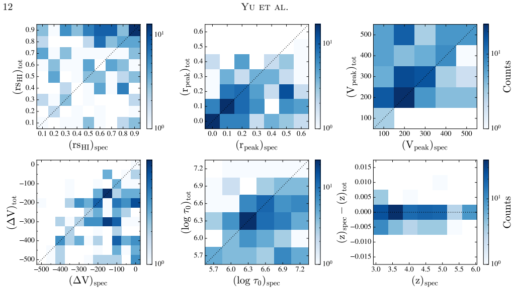
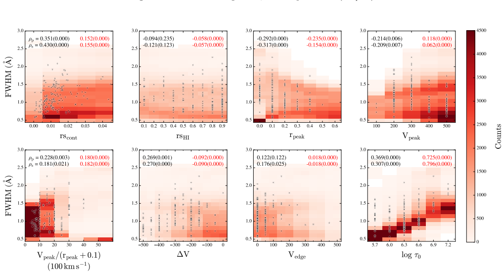
On the paper's own terms, the central discovery is that the spectra and surface brightness profiles of 163 red-peak-dominated Lyα emitters in the MUSE Hubble Ultra Deep Field are all approximately reproduced by one six-parameter expanding-halo model, and that the best-fit values concentrate at $r_{\mathrm{s,HI}} = 0.9\,r_{\mathrm{max}}$ and $V_{\mathrm{edge}} = 0$ km/s. The authors interpret this pile-up as showing that the hydrogen medium around these galaxies is extended and essentially static at large radii, and they show that this conclusion can only be reached when spectra and surface brightness profiles are modelled together: fitting either observable alone leaves the parameters poorly determined. A correlation analysis then connects observables to physical parameters, showing that Lyα halo size tracks the medium and source scale radii, whereas spectral peak shift and FWHM track optical depth, with outflow kinematics modulating the trends and adding scatter.
Load-bearing premise
The conclusion depends on the assumption that the true best fit for each galaxy lies inside the chosen parameter grid, since the best-fit values of $r_{\mathrm{s,HI}}$ and $V_{\mathrm{edge}}$ sit exactly at the grid boundary and the paper does not test whether extending the grid changes the result.
Editorial extensions
If this is right
- If the claim holds, halo size measurements from Lyα surface brightness maps can be translated into physical gas and stellar extents for large samples, without needing expensive hydrodynamical simulations.
- The best-fit pile-up at large $r_{\mathrm{s,HI}}$ and low $V_{\mathrm{edge}}$ implies that outflow deceleration zones, where gas returns to near rest at large radii, are common in the circumgalactic medium of z=3–6 star-forming galaxies.
- Because spectrum-only or SBP-only fits scatter much more than joint fits, future Lyα surveys should treat spectral and spatial data as a single constraint set; conclusions drawn from either alone will be unreliable.
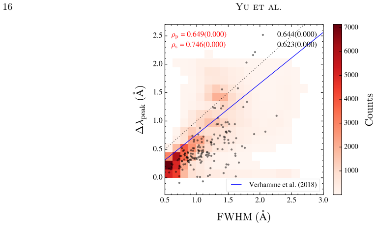
- The peak-shift–FWHM relation commonly used to estimate systemic redshifts is shown to be sample-dependent: red-peak-only galaxies and double-peaked galaxies occupy different regions of that plane, so the relation needs velocity-profile information to be predictive.
Reading between the lines
- If the adopted grid had allowed $r_{\mathrm{s,HI}}$ beyond $0.9\,r_{\mathrm{max}}$ and $V_{\mathrm{edge}}$ below 0 km/s, the best fits might have moved further out and further down, making the paper's physical conclusion a lower limit on gas extent rather than a measurement.
- The authors neglect IGM transmission, which is strongest at z≈6, so the low-velocity edge could partly absorb blue-wing photons; a natural extension is to fold in per-object IGM transmission to see whether the $V_{\mathrm{edge}}$ distribution shifts.
- The same joint-fitting machinery could be applied to double-peaked LAEs, spectroscopically confirmed redshifts, or higher-signal-to-noise IFU data to test whether the pile-up persists with independent data.
Editorial analysis
A structured set of objections, weighed in public.
Referee Report
Summary. Yu et al. model the Lyα spectra and surface brightness profiles (SBPs) of 163 MUSE Lyα-emitting galaxies at z=3–6 using the six-parameter expanding-halo Monte Carlo radiative transfer model of Song et al. (2020). They find that the best-fit models reproduce both observables for most galaxies, and that the simultaneous best-fit values of the HI density scale radius rsHI cluster at 0.9 rmax and the outer-edge velocity Vedge at 0 km/s, which they interpret as evidence for a broad, nearly static outer circumgalactic medium. They further analyze correlations between observables and model parameters, concluding that the spatial extent of Lyα halos is primarily set by the medium and source scale radii, while spectral peak shift and FWHM are mainly governed by optical depth with a secondary role for the velocity structure. The paper also shows that correlations derived from the full model grid and from the best-fit subset differ substantially, and it cautions against overinterpreting the full-grid correlations.
Significance. If the central claim holds, this paper demonstrates that a simple parametric outflow model can simultaneously reproduce Lyα spectra and SBPs for a statistically meaningful sample, extending Song et al. (2020) from 8 to 163 galaxies and placing population-level constraints on the CGM of z=3–6 LAEs. The use of direct MUSE data rather than digitized figures, the systematic MLE-versus-MAP comparison, and the explicit discussion of sample bias in correlation analysis are notable strengths that increase confidence in the fitting procedure. However, the interpretation that the outer medium is broad and static rests on best-fit parameters that pile up at the edge of the adopted parameter grid, and on the neglect of IGM transmission at redshifts where it is known to be important; both issues are load-bearing for the central conclusion and require further testing.
major comments (2)
- [Section 4.2, Table 1, Figure 10] The best-fit rsHI values for the simultaneous fits concentrate at 0.9 rmax, which is the upper boundary of the adopted grid (rsHI ∈ {0.1, ..., 0.9}). The paper interprets this pile-up as evidence that the medium is 'largely extended', but a pile-up at a grid boundary is also what one expects if the true best fit lies beyond the searched range. No test with rsHI > 0.9 or with a larger rmax is presented, so the MLE at 0.9 cannot be taken as a reliable estimate of the preferred scale radius. Because this is one of the two pillars of the central 'broad static medium' claim, the authors should either extend the grid and show the likelihood behavior beyond the boundary, or explicitly qualify rsHI = 0.9 as a lower limit rather than a detection. The qualitative direction of the claim may survive such a test, but the current analysis does not demonstrate it.
- [Section 3, paragraph beginning 'It is worth noting...'] The models ignore IGM transmission even though the sample spans z=3–6, where the mean IGM transmission declines from roughly 60% at z=3 to near zero at z=6 (Inoue et al. 2014). The model has no physical mechanism other than outflowing gas to suppress the blue Lyα peak, so IGM absorption can produce red-peak-dominated spectra even for intrinsically symmetric or weakly outflowing media. This degeneracy may bias the inferred velocity structure, notably Vedge, and possibly rsHI for the highest-redshift objects. The authors acknowledge the issue but do not quantify its impact. I request a quantitative check, such as applying a representative IGM transmission to the model spectra for a subsample and refitting, or at least a careful discussion of how the central conclusion of a static outer CGM is robust to plausible IGM attenuation.
minor comments (5)
- [Section 2] The text states that 19 of 184 LAEs have double-peaked spectra and the rest have red-peak-only spectra, which would leave 165 red-peak-dominated objects, yet the modeling is performed for 163 galaxies; please clarify why two additional galaxies were excluded.
- [Section 3, Equation (1) and following paragraph] The text says 'the total likelihood was computed by summing the likelihoods calculated from the spectrum and SBP,' but Equation (1) defines a log-likelihood. If the sum is over log-likelihoods, the wording should say so; if the sum is actually over likelihoods (not log-likelihoods), the statistical procedure is incorrect and needs correction.
- [Section 4.2, Figure 10] Vedge = Vpeak + ΔV is introduced only in the Figure 10 axis label; it would be clearer to define this derived quantity explicitly in the text before discussing its best-fit distribution.
- [Section 4.1, Figure 4] The reduced chi-square values are discussed without specifying how the degrees of freedom are computed for each object; because the number of spectral and SBP data points varies and parameters are selected on a discrete grid, a brief definition of the reduced chi-square would improve interpretability.
- [Figures 11–14] Several correlation p-values are printed as 0.000; these should be reported as <0.001 or as the actual floating-point values to avoid implying a literally zero probability.
Circularity Check
No circularity: the paper fits an independently published radiative-transfer model to external MUSE observations; the self-citations are normal model reuse and do not reduce the conclusions to inputs.
full rationale
The derivation chain starts from the Song et al. (2020) MCRT calculations, which are used as a forward generative model. Best-fit parameters are obtained by comparing model spectra and SBPs to MUSE observations from Leclercq et al. (2017), an external dataset, through the likelihood in Eq. (1). The central claims (broad HI distribution, low Vedge, and the correlations of halo size with rsHI and rscont) are interpretations of fitted parameters and of the forward-model grid, not quantities defined in terms of the targets they are said to explain. The pile-up of rsHI at the upper grid boundary 0.9 rmax is a search-range completeness limitation that could affect the physical interpretation, but it does not make the conclusion equivalent by construction to the input; one would need to show that the likelihood itself, not the grid edge, selected that value. The self-citation to Song et al. (2020) is standard reuse of a previously published model, and the present paper applies it to a new, larger external MUSE sample while also comparing against the original eight objects, so the citation is not load-bearing in a circular sense. No parameter is fitted to a subset and then relabeled as a prediction, no uniqueness theorem is imported from the authors' prior work, and no empirical pattern is merely renamed. The paper is therefore self-contained against external benchmarks for the purpose of this analysis, and no significant circularity is found.
Assumptions & free parameters
free parameters (6)
- rsHI (HI density scale radius, normalized by rmax) =
grid 0.1 to 0.9; best-fit pile-up at 0.9
- rpeak (radius of peak outflow velocity) =
grid 0.0 to 0.6
- Vpeak (peak outflow velocity) =
grid 100 to 500 km/s
- ΔV (velocity difference at rpeak and edge) =
grid -500 to 0 km/s
- log τ0 (log optical depth at Lyα center) =
grid 5.7 to 7.2
- z (redshift offset from MUSE estimate) =
grid zMUSE -0.015 to +0.002
assumptions (6)
- domain assumption The circumgalactic medium is spherically symmetric with an exponential HI density profile of scale radius rsHI.
- domain assumption The medium is isothermal at 10^4 K.
- domain assumption The bulk motion is a smooth outflow that rises linearly to Vpeak at rpeak and then drops to Vpeak+ΔV at rmax.
- domain assumption The initial Lyα photon distribution follows the UV continuum distribution, an exponential in projection and a modified Bessel function in 3D.
- ad hoc to paper Dust-to-gas ratio is zero and the intergalactic medium is ignored.
- ad hoc to paper The parameter grid boundaries (rsHI max 0.9, Vedge max 0) encompass the true best-fit parameters.
Cite this review
Pith. "Pith review of Ly$\alpha$ radiative transfer modeling for 163 MUSE Ly$\alpha$-emitting galaxies at $z=$3--6." pith.science (2026). https://pith.science/paper/PHXCQVXD
@misc{pith2026250608290,
  author       = {Pith},
  title        = {Pith review of: Ly$\alpha$ radiative transfer modeling for 163 MUSE Ly$\alpha$-emitting galaxies at $z=$3--6},
  year         = {2026},
  howpublished = {\url{https://pith.science/paper/PHXCQVXD}},
  note         = {Machine review of arXiv:2506.08290}
}
abstract
We utilized Ly$\alpha$ radiative transfer calculations from \citet{Song2020} to investigate the properties of extended Ly$\alpha$ halos around star-forming galaxies in the \textit{Hubble} Ultra Deep Field, observed by the Multi-Unit Spectroscopic Explorer. Expanding on the work of \citet{Song2020}, which was limited to eight galaxies, we derived best-fit models for a significantly larger sample of 163 galaxies, which successfully reproduced both their Ly$\alpha$ spectra and surface brightness profiles (SBPs). These best-fit models suggest a broad medium distribution surrounding each galaxy, with low expanding velocities at large radii. This conclusion could not have been drawn from modeling either the spectrum or SBP alone, but only through simultaneous modeling of both. Our correlation analysis between observables and model parameters reveals that the spatial extent of Ly$\alpha$ halos is primarily determined by the extents of the medium and the source, while the spectral peak shift and full width at half maximum are governed mainly by optical depth, with the velocity structure of the medium playing a secondary yet non-negligible role. The fact that various correlations derived from the full set of models and those from the best-fit subset can differ significantly highlights the complex and interdependent nature of Ly$\alpha$ radiative transfer. All model parameters interact to shape the observed Ly$\alpha$ features in a non-trivial way.
Figures


Figures from the paper (11 more)




Reference graph
Works this paper leans on
-
[1]
Ahn, S.-H., Lee, H.-W., & Lee, H. M. 2003, MNRAS, 340, 863, doi: 10.1046/j.1365-8711.2003.06353.x
arXiv 2003
-
[2]
2010, in Society of Photo-Optical Instrumentation Engineers (SPIE) Conference Series, Vol
Bacon, R., Accardo, M., Adjali, L., et al. 2010, in Society of Photo-Optical Instrumentation Engineers (SPIE) Conference Series, Vol. 7735, Ground-based and Airborne Instrumentation for Astronomy III, ed. I. S. McLean, S. K. Ramsay, & H. Takami, 773508, doi: 10.1117/12.856027
-
[3]
2015, A&A, 575, A75, doi: 10.1051/0004-6361/201425419
Bacon, R., Brinchmann, J., Richard, J., et al. 2015, A&A, 575, A75, doi: 10.1051/0004-6361/201425419
-
[4]
Barnes, L. A., Garel, T., & Kacprzak, G. G. 2014, PASP, 126, 969, doi: 10.1086/679178
doi:10.1086/679178 2014
-
[5]
2014, A&A, 572, A74, doi: 10.1051/0004-6361/201424755
Behrens, C., & Braun, H. 2014, A&A, 572, A74, doi: 10.1051/0004-6361/201424755
-
[6]
2023, MNRAS, 523, 3749, doi: 10.1093/mnras/stad1523
Blaizot, J., Garel, T., Verhamme, A., et al. 2023, MNRAS, 523, 3749, doi: 10.1093/mnras/stad1523
-
[7]
2011, Nature, 476, 288, doi: 10.1038/476288a
Bower, R. 2011, Nature, 476, 288, doi: 10.1038/476288a
-
[8]
2023, ApJ, 945, 100, doi: 10.3847/1538-4357/acac98
Chang, S.-J., Yang, Y., Seon, K.-I., Zabludoff, A., & Lee, H.-W. 2023, ApJ, 945, 100, doi: 10.3847/1538-4357/acac98
Show all 43 references
-
[9]
2014, PASA, 31, e040, doi: 10.1017/pasa.2014.33
Dijkstra, M. 2014, PASA, 31, e040, doi: 10.1017/pasa.2014.33
2014 doi
-
[10]
2006, ApJ, 649, 14, doi: 10.1086/506243
Dijkstra, M., Haiman, Z., & Spaans, M. 2006, ApJ, 649, 14, doi: 10.1086/506243
2006 doi
-
[11]
2021, MNRAS, 504, 1902, doi: 10.1093/mnras/stab990
Garel, T., Blaizot, J., Rosdahl, J., et al. 2021, MNRAS, 504, 1902, doi: 10.1093/mnras/stab990
2021 doi
-
[12]
2017, VizieR Online Data Catalog: 237 Lyman-alpha spectra of MUSE-Wide survey (Gronke, 2017), VizieR On-line Data Catalog: J/A+A/608/A139
Gronke, M. 2017, VizieR Online Data Catalog: 237 Lyman-alpha spectra of MUSE-Wide survey (Gronke, 2017), VizieR On-line Data Catalog: J/A+A/608/A139. Originally published in: 2017A&A...608A.139G, doi: 10.26093/cds/vizier.36080139
2017 doi
-
[13]
2015, ApJ, 812, 123, doi: 10.1088/0004-637X/812/2/123
Gronke, M., Bull, P., & Dijkstra, M. 2015, ApJ, 812, 123, doi: 10.1088/0004-637X/812/2/123
2015 doi
-
[14]
2016, ApJ, 826, 14, doi: 10.3847/0004-637X/826/1/14
Gronke, M., & Dijkstra, M. 2016, ApJ, 826, 14, doi: 10.3847/0004-637X/826/1/14
2016 doi
-
[15]
Gronke, M., Dijkstra, M., McCourt, M., & Oh, S. P. 2017, A&A, 607, A71, doi: 10.1051/0004-6361/201731013
2017 doi
-
[16]
Hansen, M., & Oh, S. P. 2006, MNRAS, 367, 979, doi: 10.1111/j.1365-2966.2005.09870.x
2006
-
[17]
2015, PASA, 32, e027, doi: 10.1017/pasa.2015.25
Hayes, M. 2015, PASA, 32, e027, doi: 10.1017/pasa.2015.25
2015 doi
-
[18]
2011, Nature, 476, 304, doi: 10.1038/nature10320
Hayes, M., Scarlata, C., & Siana, B. 2011, Nature, 476, 304, doi: 10.1038/nature10320
2011 doi
-
[19]
K., Shimizu, I., Iwata, I., & Tanaka, M
Inoue, A. K., Shimizu, I., Iwata, I., & Tanaka, M. 2014, MNRAS, 442, 1805, doi: 10.1093/mnras/stu936
2014 doi
-
[20]
2020, ApJ, 894, 33, doi: 10.3847/1538-4357/ab837f
Kim, E., Yang, Y., Zabludoff, A., et al. 2020, ApJ, 894, 33, doi: 10.3847/1538-4357/ab837f
2020 doi
-
[21]
A., Zheng, Z., Dav´ e, R., et al
Kollmeier, J. A., Zheng, Z., Dav´ e, R., et al. 2010, ApJ, 708, 1048, doi: 10.1088/0004-637X/708/2/1048
2010 doi
-
[22]
2007, ApJL, 657, L69, doi: 10.1086/513191
Laursen, P., & Sommer-Larsen, J. 2007, ApJL, 657, L69, doi: 10.1086/513191
2007 doi
-
[23]
2017, A&A, 608, A8, doi: 10.1051/0004-6361/201731480
Leclercq, F., Bacon, R., Wisotzki, L., et al. 2017, A&A, 608, A8, doi: 10.1051/0004-6361/201731480
2017 doi
-
[24]
2022, MNRAS, 513, 5034, doi: 10.1093/mnras/stac1207
Li, Z., & Gronke, M. 2022, MNRAS, 513, 5034, doi: 10.1093/mnras/stac1207
2022 doi
-
[25]
Neufeld, D. A. 1990, ApJ, 350, 216, doi: 10.1086/168375
1990 doi
-
[26]
2021, ApJ, 922, 263, doi: 10.3847/1538-4357/ac2f4b
Park, H., Jung, I., Song, H., et al. 2021, ApJ, 922, 263, doi: 10.3847/1538-4357/ac2f4b
2021 doi
-
[27]
Prescott, M. K. M., Smith, P. S., Schmidt, G. D., & Dey, A. 2011, ApJL, 730, L25, doi: 10.1088/2041-8205/730/2/L25
2011 doi
-
[28]
2011, A&A, 531, A12, doi: 10.1051/0004-6361/201116709
Schaerer, D., Hayes, M., Verhamme, A., & Teyssier, R. 2011, A&A, 531, A12, doi: 10.1051/0004-6361/201116709
2011 doi
-
[29]
2020, ApJS, 250, 9, doi: 10.3847/1538-4365/aba2d6
Seon, K.-I., & Kim, C.-G. 2020, ApJS, 250, 9, doi: 10.3847/1538-4365/aba2d6
2020 doi
-
[30]
2022, ApJS, 259, 3, doi: 10.3847/1538-4365/ac3af1
Seon, K.-I., Song, H., & Chang, S.-J. 2022, ApJS, 259, 3, doi: 10.3847/1538-4365/ac3af1
2022 doi
-
[31]
2019, MNRAS, 484, 39, doi: 10.1093/mnras/sty3483
Smith, A., Ma, X., Bromm, V., et al. 2019, MNRAS, 484, 39, doi: 10.1093/mnras/sty3483
2019 doi
-
[32]
2015, MNRAS, 449, 4336, doi: 10.1093/mnras/stv565 18Yu et al
Smith, A., Safranek-Shrader, C., Bromm, V., & Milosavljevi´ c, M. 2015, MNRAS, 449, 4336, doi: 10.1093/mnras/stv565 18Yu et al
2015 doi
-
[33]
2022, MNRAS, 517, 1, doi: 10.1093/mnras/stac2641
Smith, A., Kannan, R., Tacchella, S., et al. 2022, MNRAS, 517, 1, doi: 10.1093/mnras/stac2641
2022 doi
-
[34]
Song, H., Seon, K.-I., & Hwang, H. S. 2020, ApJ, 901, 41, doi: 10.3847/1538-4357/abac02
2020 doi
-
[35]
2012, A&A, 546, A111, doi: 10.1051/0004-6361/201218783
Verhamme, A., Dubois, Y., Blaizot, J., et al. 2012, A&A, 546, A111, doi: 10.1051/0004-6361/201218783
2012 doi
-
[36]
2006, A&A, 460, 397, doi: 10.1051/0004-6361:20065554
Verhamme, A., Schaerer, D., & Maselli, A. 2006, A&A, 460, 397, doi: 10.1051/0004-6361:20065554
2006 doi
-
[37]
2018, MNRAS, 478, L60, doi: 10.1093/mnrasl/sly058
Verhamme, A., Garel, T., Ventou, E., et al. 2018, MNRAS, 478, L60, doi: 10.1093/mnrasl/sly058
2018 doi
-
[38]
2016, A&A, 587, A98, doi: 10.1051/0004-6361/201527384
Wisotzki, L., Bacon, R., Blaizot, J., et al. 2016, A&A, 587, A98, doi: 10.1051/0004-6361/201527384
2016 doi
-
[39]
2016, ApJ, 820, 130, doi: 10.3847/0004-637X/820/2/130
Yang, H., Malhotra, S., Gronke, M., et al. 2016, ApJ, 820, 130, doi: 10.3847/0004-637X/820/2/130
2016 doi
-
[40]
E., et al
Yang, H., Malhotra, S., Rhoads, J. E., et al. 2017, ApJ, 838, 4, doi: 10.3847/1538-4357/aa6337
2017 doi
-
[41]
2017, ApJ, 834, 182, doi: 10.3847/1538-4357/834/2/182
You, C., Zabludoff, A., Smith, P., et al. 2017, ApJ, 834, 182, doi: 10.3847/1538-4357/834/2/182
2017 doi
-
[42]
2011, ApJ, 739, 62, doi: 10.1088/0004-637X/739/2/62
Zheng, Z., Cen, R., Weinberg, D., Trac, H., & Miralda-Escud´ e, J. 2011, ApJ, 739, 62, doi: 10.1088/0004-637X/739/2/62
2011 doi
-
[43]
2002, ApJ, 578, 33, doi: 10.1086/342400
Zheng, Z., & Miralda-Escud´ e, J. 2002, ApJ, 578, 33, doi: 10.1086/342400
2002 doi
Reviewed August 7, 2026 · model on record in the stance chip above.
Discussion (0). Sign in to comment.