REVIEW 3 major objections 6 minor 59 references
Guidelines for LASSO and derivatives use under different dependence and scale structures
T0 review · 3 major / 6 minor · reviewed 2026-08-07 · deepseek-v4-flash
Pith's one-line read The paper argues that the best LASSO-type procedure depends jointly on dependence structure, scale structure, and the practitioner's objective, and that univariate standardization is not uniformly beneficial.
desk verdict A careful, useful simulation study on when univariate standardization helps or hurts LASSO under dependence and scale; the main caveat is that the guidelines generalize beyond Toeplitz designs without evidence. read the letter →
The pith
A machine-rendered reading of the paper's core claim, the machinery that carries it, and where it could break.
The reading
What carries the argument
The machinery is the side-by-side comparison of the raw centered design matrix Xr and its univariate standardized version Xus across simulated Gaussian designs whose covariance is diagonal or Toeplitz, with relevant covariates placed in blocks or spread sparsely and with scale variations applied to relevant or noisy covariates. In the orthogonal case, the paper shows that selection depends on the covariate variance and the inner product with the standardized covariate, making scale an explicit selection driver; in non-orthogonal designs no closed-form LASSO solution exists, so dependence and scale interact through the correlation structure. The final decision tree translates the simulation outcomes into method recommendations indexed by dependence (yes/no), scale differences (yes/no), and objective (false discovery proportion, true positive proportion, good-interval MSE, or overestimation correction).
What would settle it
Simulate or collect data with a dependence structure outside the Toeplitz family — for example, a block-diagonal or factor covariance with non-Gaussian errors and the same scale patterns as RNC.TOEP-S — and compare the decision tree's recommendation against raw and standardized LASSO variants; if the recommended method is not the best in selection or prediction, the guidelines fail.
Extended reading notes
Core claim
On the paper's own terms, the central discovery is that univariate standardization is not a harmless preprocessing step: it changes which covariates the LASSO selects, and the direction of the change is governed by the dependence-scale configuration. In the orthogonal IND scenarios, raw and standardized data behave similarly, and standardization chiefly reduces scale-driven false discoveries among noisy high-variance covariates. In the unit-scale Toeplitz scenarios (UTOEP-B, UTOEP-S) the two preprocessing choices again behave similarly, with strong correlation (rho=0.9) making a conservative subset-selection strategy competitive with full recovery. In the scale-mixed Toeplitz scenarios (RC.TOEP-S, RNC.TOEP-S) the two failure modes separate: raw-data LASSO is confused by high-scale noisy covariates, while univariate standardization disrupts the dependence structure and adds more noise at a similar rate of relevant-covariate recovery. The authors conclude that method choice should be driven jointly by dependence structure, scale structure, sample regime, and the objective of selection versus prediction.
Load-bearing premise
The load-bearing premise is that the Gaussian diagonal and Toeplitz simulation scenarios are representative enough that the decision tree transfers to arbitrary high-dimensional linear regression problems with dependence and scale variation.
Editorial extensions
If this is right
- Under strong Toeplitz dependence, methods that exploit the dependence structure (AdapL.1se, Dant, DC.VS) can select a small representative subset of relevant covariates with few false discoveries, instead of forcing full recovery of the true support.
- In scale-mixed Toeplitz settings, raw-data LASSO tends to be confused by noisy high-scale covariates, and univariate standardization does not remove the confusion: it disrupts dependence and adds more noise while recovering about the same number of relevant terms.
- Prediction-oriented users should not expect LASSO-type methods to report honest accuracy: most overestimate predictive performance, and only some variants (notably LASSO.1se and LASSO.BIC at n=300) fall into the good-MSE interval in the studied scenarios.
- Under independence, univariate standardization is mainly a safeguard against scale-driven false discoveries, and raw and standardized selections are otherwise close.
- The paper's decision tree offers a concrete starting point: choose the method according to dependence (yes/no), scale differences (yes/no), sample regime (p>n or n>p), and whether the goal is minimizing false discoveries, maximizing true positives, obtaining good prediction error, or correcting overestimation.
Reading between the lines
- A natural extension the paper does not pursue is a quantitative threshold for when standardization hurts: the simulations suggest the harm grows with the correlation between relevant and noisy covariates and with the scale gap, but no formula is given.
- Because the scenarios are confined to Gaussian diagonal/Toeplitz designs, the decision tree's transfer to block-structured or factor-model dependence, non-Gaussian errors, or data with unknown support locations remains untested; applying the tree as a general recipe would be an extrapolation.
- Practitioners could use the paper's results to justify a stability check: fit both raw and standardized versions on a subsample and compare selection agreement, since either preprocessing can win depending on the configuration.
- The evidence that a few high-correlation covariates can explain most variability suggests that the notion of 'true support' may be less decision-relevant under strong dependence than a parsimonious predictive set, which is a perspective the paper raises implicitly in its representative-subset discussion.
Editorial analysis
A structured set of objections, weighed in public.
Referee Report
Summary. The paper investigates the effect of univariate standardization on the LASSO and several competitors (adaptive LASSO, SCAD, Dantzig selector, relaxed LASSO, square-root LASSO, scaled LASSO, and distance-covariance variable selection) in high-dimensional linear regression settings where covariates exhibit dependence and heterogeneous scales. A simulation study with p=100, n=25-300, and covariance structures that are diagonal, Toeplitz (rho=0.5, 0.9), and Toeplitz with added scale perturbations compares raw versus univariately standardized data on two criteria: variable selection (false discovery proportion and true positive proportion) and prediction (MSE relative to a 'Good Interval' and overestimation behavior). The paper concludes with a decision tree (Figure 14) recommending procedures by dependence/scale configuration and objective, and applies the methods to three real datasets.
Significance. The central qualitative finding is useful and convincingly demonstrated within the simulated designs: univariate standardization is not uniformly beneficial, because in dependence settings it can disrupt the dependence structure and add noise, while raw data are vulnerable to large-scale noisy covariates. The paper's strengths include the breadth of competitors, the explicit separation of selection and prediction objectives, the availability of code on GitHub, and the honest acknowledgment in Figure 14's footnote that the recommendation depends on the type of dependence structure. If the scope were appropriately restricted and the real-data prediction protocol corrected, the guidelines could serve as a practical reference. However, as written, the external validity of the decision tree beyond the simulated covariance families is not established, and the real-data predictive comparisons are compromised by the evaluation protocol.
major comments (3)
- [Section 7 / Figure 14] The decision tree dichotomizes 'dependence' (Yes/No) and 'scales' (Yes/No) and then gives concrete procedure recommendations for every branch, but the simulation evidence covers only diagonal and Toeplitz Gaussian designs (Section 3) with fixed support locations and coefficient magnitudes. The footnote '(*) It depends on the type of dependence structure' concedes this limitation, but the tree still presents the recommendations as applying to all dependence structures. Since the LASSO's selection behavior under dependence is governed by quantities like the irrepresentable condition and coherence, which can vary substantially within the 'dependence = Yes' category, the guidelines need either to be explicitly restricted to Toeplitz-type dependence with a clear operational definition, or to be validated on additional covariance families (e.g., equicorrelation, factor models, or negative-correlation structures). As written, the title and Section 7 overstate the scope of the findings.
- [Sections 6.1-6.3] The real-data prediction protocol selects covariates using the full dataset before splitting into training and test sets; for example, Section 6.1 states: 'First, the relevant covariates are selected employing the total n = 71 samples. Subsequently, the sample is randomly divided in two...'. This is a data-leakage protocol: the test set influences covariate selection, so the reported MSE and %Dev values in Tables 11-13 are optimistic and the comparisons among methods are not honest out-of-sample evaluations. The selection step should be nested inside the training folds (e.g., repeated cross-validation) or performed on the training portion only for each split. Because the real-data analysis is a stated contribution of the paper, this protocol issue is load-bearing and should be corrected.
- [Sections 4-5 (all simulation tables)] All simulation results are reported as point estimates over M=500 replicates without standard errors or confidence intervals. For example, in Table 5 the RAW versus UNIV MSE differences for LASSO.1se (12.624 vs 7.092 in RC.IND; 12.366 vs 6.806 in RNC.IND) are large, but in Table 1 differences such as 1.345 vs 1.346 are clearly negligible; without a measure of Monte Carlo error the reader cannot assess which differences are meaningful. Given that the guidelines in Figure 14 aggregate across many scenario cells, the authors should report Monte Carlo standard errors or display variability (e.g., boxplots) for at least the key scenarios. This would substantially strengthen the evidential basis for the qualitative recommendations.
minor comments (6)
- [Section 1] The text says 'an independent and identically distributed (idd) sample'; 'idd' should be 'iid'.
- [Section 4] The typo 'Topelitz covariance structure' should read 'Toeplitz covariance structure'.
- [Section 6.3] Table 13's caption says 'training sample of size 191' but the text says the training sample is 1215 observations; the caption should match the narrative.
- [Section 6.1] The sentence 'Results for Xus are displayed in Table 11, while those concerning Xr are collected in Table 11 in Section E.4.1' has a duplicate table number; the Xr table is presumably Table 27 in the appendix and should be cited correctly.
- [Section 2, Eq. (2)] The statement 'keeping just the orthogonal assumption of X' is ambiguous because Eq. (2) also assumes the columns of X have equal norm; the authors should explicitly state that the formula holds for orthogonal (not necessarily unit-norm) columns and define sigma_j^2 as the column norm squared.
- [Section 3] The condition written as 'n > log(p)s ≈ 4.61s' is imprecise; it should be expressed as n > s log p (with the relevant constant) and the associated references for the consistent-selection condition should be stated more carefully.
Circularity Check
No significant circularity: guidelines are empirical summaries tested on real data; self-citations are contextual only.
full rationale
This paper is an empirical simulation study rather than a derivation, and the only closed-form result, equation (2), is a standard orthonormal-LASSO formula cited to Giraud (2014); it is used only to motivate the scale effect and is not the source of the later guidelines. The recommendations in Figure 14 are explicit post hoc summaries of the Monte Carlo results over the Section 3 grid, with the footnote '(*) It depends on the type of dependence structure' acknowledging the limits of the dependence branch, so the tree is not a prediction that reduces to its own inputs by construction. No parameter is fitted to one part of the data and then renamed a prediction; the oracle MSE and GI comparisons are independent evaluation criteria against known simulation truth, and the three real datasets supply an external, albeit qualitative, check. The repeated citations to Freijeiro-González et al. (2022) and Febrero-Bande et al. (2019) are for background, implementation details, and competitor definitions; the Xr-versus-Xus comparisons are computed in this paper using glmnet and are not justified by those citations. The main risk is external validity of the Gaussian diagonal/Toeplitz scenario grid, which is a generality limitation rather than a circularity.
Assumptions & free parameters
free parameters (5)
- Signal coefficients beta =
1.25 (IND), 0.5 (UTOEP and TOEP-S)
- Scale values in design covariance =
0.5, 1, 3, 10, 25, 50
- Dependence strength rho =
0.5, 0.9
- Noise variance sigma_epsilon =
derived so 90% of deviance is explained
- Number and location of relevant covariates s =
10 (IND, UTOEP-S, TOEP-S), 15 (UTOEP-B)
assumptions (4)
- domain assumption The data generating process is a centered linear regression Y = X beta + epsilon with no intercept (Sections 1 and 3).
- domain assumption Covariates are Gaussian, X ~ N(0, Sigma), with diagonal or Toeplitz covariance (Section 3).
- standard math The beta-min and n > s log(p) conditions from Buhlmann and Van De Geer (2011) guide the choice of simulation parameters (Section 3).
- domain assumption Cross-validated glmnet with 10 folds and a grid of length 100 is a fair implementation basis for comparing all methods (Section 4).
Cite this review
Pith. "Pith review of Guidelines for LASSO and derivatives use under different dependence and scale structures." pith.science (2026). https://pith.science/paper/V4ZBKVSG
@misc{pith2026250608582,
  author       = {Pith},
  title        = {Pith review of: Guidelines for LASSO and derivatives use under different dependence and scale structures},
  year         = {2026},
  howpublished = {\url{https://pith.science/paper/V4ZBKVSG}},
  note         = {Machine review of arXiv:2506.08582}
}
abstract
In a multivariate linear regression model with $p>1$ covariates, implementation of penalization techniques often implies a preliminary univariate standardization step. Although this prevents scale effects on the covariates selection procedure, possible dependence structures can be disrupted, leading to wrong results. This is particularly challenging in high-dimensional settings where $p \geq n$. In this paper, we analyze the standardization effect on the LASSO for different dependence-scales contexts by means of an extensive simulation study. Two distinct objectives are pursued: adequate covariate selection and proper predictive capability. Additionally, its behavior is compared with the one of some well-known or innovative competitors. This comparison is also extended to three real datasets facing different dependence-scales patterns. Eventually, we conclude with discussion and guidelines on the most suitable methodology for each case in terms of covariates selection or prediction.
Figures
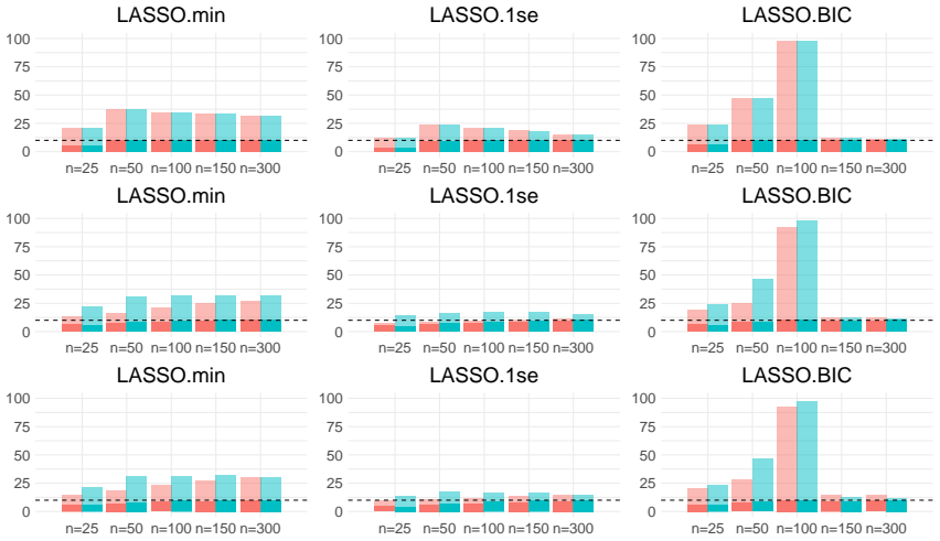


Figures from the paper (11 more)




Reference graph
Works this paper leans on
-
[1]
Ali, A. and Tibshirani, R. J. (2019). The Generalized Lasso Problem and Uniqueness . Electronic Journal of Statistics , 13(2):2307 -- 2347
work page 2019
-
[2]
Belloni, A. and Chernozhukov, V. (2013). Least squares after model selection in high-dimensional sparse models . Bernoulli , 19(2):521 -- 547
work page 2013
-
[3]
Belloni, A., Chernozhukov, V., and Wang, L. (2011). Square-root lasso: Pivotal recovery of sparse signals via conic programming. Biometrika , 98(4):791--806
work page 2011
-
[4]
Bogdan, M., Van Den Berg, E., Sabatti, C., Su, W., and Cand \`e s, E. J. (2015). SLOPE -adaptive variable selection via convex optimization. The Annals of Applied Statistics , 9(3):1103
work page 2015
-
[5]
Breheny, P. and Huang, J. (2011). Coordinate descent algorithms for nonconvex penalized regression, with applications to biological feature selection. The Annals of Applied Statistics , 5(1):232--253
work page 2011
-
[6]
B \"u hlmann, P. and Van De Geer, S. (2011). Statistics for High-Dimensional Data: Methods, Theory and Applications . Springer Science & Business Media
work page 2011
-
[7]
Bunea, F. (2008). Honest variable selection in linear and logistic regression models via l1 and l1 + l2 penalization. Electronic Journal of Statistics , 2
work page 2008
-
[8]
Bühlmann, P., Kalisch, M., and Meier, L. (2014). High-dimensional statistics with a view toward applications in biology. Annual Review of Statistics and Its Application , 1(1):255--278
work page 2014
Show all 59 references
-
[9]
and Tao, T
Candès, E. and Tao, T. (2007). The D antzig selector: Statistical estimation when p is much larger than n . The Annals of Statistics , 35(6):2313--2351
2007
-
[10]
Cortez, P., Cerdeira, A., Almeida, F., Matos, T., and Reis, J. (2009). Modeling wine preferences by data mining from physicochemical properties. Decision Support Systems , 47(4):547--553. Smart Business Networks: Concepts and Empirical Evidence
2009
-
[11]
S., Hebiri, M., and Lederer, J
Dalalyan, A. S., Hebiri, M., and Lederer, J. (2017). On the prediction performance of the Lasso . Bernoulli , 23(1):552 -- 581
2017
-
[12]
Dezeure, R., B\"uhlmann, P., Meier, L., and Meinshausen, N. (2015). High-dimensional inference: Confidence intervals, p-values and R -software hdi . Statistical Science , 30(4):533--558
2015
-
[13]
Draper, N. R. and Smith, H. (1998). Applied Regression Analysis . John Wiley & Sons, Ltd
1998
-
[14]
Fan, J. (1997). Comments on wavelets in statistics: A review by A. Antoniadis . Journal of the Italian Statistical Society , 6(2):131
1997
-
[15]
and Li, R
Fan, J. and Li, R. (2001). Variable selection via nonconcave penalized likelihood and its oracle properties. Journal of the American Statistical Association , 96(456):1348--1360
2001
-
[16]
and Lv, J
Fan, J. and Lv, J. (2008). Sure independence screening for ultrahigh dimensional feature space. Journal of the Royal Statistical Society: Series B (Statistical Methodology) , 70(5):849--911
2008
-
[17]
Febrero-Bande, M., Gonz \'a lez-Manteiga, W., and Oviedo de la Fuente, M. (2019). Variable selection in functional additive regression models. Computational Statistics , 34(2):469--487
2019
-
[18]
and Oviedo de la Fuente , M
Febrero-Bande, M. and Oviedo de la Fuente , M. (2012). Statistical computing in functional data analysis: The R package fda.usc . Journal of Statistical Software , 51(4):1--28
2012
-
[19]
Freijeiro-González, L., Febrero-Bande, M., and González-Manteiga, W. (2022). A Critical Review of LASSO and Its Derivatives for Variable Selection Under Dependence Among Covariates . International Statistical Review , 90(1):118--145
2022
-
[20]
Friedman, J., Hastie, T., and Tibshirani, R. (2000). Additive logistic regression: a statistical view of boosting (With discussion and a rejoinder by the authors) . The Annals of Statistics , 28(2):337 -- 407
2000
-
[21]
Friedman, J., Hastie, T., and Tibshirani, R. (2010). Regularization paths for generalized linear models via coordinate descent. Journal of Statistical Software , 33(1):1--22
2010
-
[22]
Friedman, J. H. (2001). Greedy function approximation: A gradient boosting machine. The Annals of Statistics , 29(5):1189 -- 1232
2001
-
[23]
Giraud, C. (2014). Introduction to High-Dimensional Statistics . Chapman and Hall/CRC
2014
-
[24]
Giraud, C., Huet, S., and Verzelen, N. (2012). High-Dimensional Regression with Unknown Variance . Statistical Science , 27(4):500 -- 518
2012
-
[25]
A., Slinker, B
Glantz, S. A., Slinker, B. K., and Neilands, T. B. (1990). Primer of applied regression and analysis of variance mcgraw-hill. Inc., New York
1990
-
[26]
Gretton, A., Bousquet, O., Smola, A., and Sch \"o lkopf, B. (2005). Measuring statistical dependence with hilbert-schmidt norms. In Jain, S., Simon, H. U., and Tomita, E., editors, Algorithmic Learning Theory , pages 63--77, Berlin, Heidelberg. Springer Berlin Heidelberg
2005
-
[27]
Hastie, T., Tibshirani, R., and Friedman, J. (2009). The Elements of Statistical Learning: Data Mining, Inference, and Prediction . Springer Science & Business Media
2009
-
[28]
Hastie, T., Tibshirani, R., and Wainwright, M. (2015). Statistical Learning with Sparsity: The Lasso and Generalizations . CRC press
2015
-
[29]
Hocking, R. R. (1983). Developments in linear regression methodology: 1959-1982. Technometrics , 25(3):219--230
1983
-
[30]
Hoerl, A. E. and Kennard, R. W. (1970). Ridge regression: Biased estimation for nonorthogonal problems. Technometrics , 12(1):55--67
1970
-
[31]
and McDonald, D
Homrighausen, D. and McDonald, D. J. (2018). A study on tuning parameter selection for the high-dimensional lasso. Journal of Statistical Computation and Simulation , 88(15):2865--2892
2018
-
[32]
Lahiri, S. N. (2021). Necessary and sufficient conditions for variable selection consistency of the LASSO in high dimensions . The Annals of Statistics , 49(2):820 -- 844
2021
-
[33]
Leng, C., Lin, Y., and Wahba, G. (2006). A note on the lasso and related procedures in model selection. Statistica Sinica , 16(4):1273--1284
2006
-
[34]
Li, X., Zhao, T., Wang, L., Yuan, X., and Liu, H. (2024). flare: Family of Lasso Regression . R package version 1.7.0.2
2024
-
[35]
Meinshausen, N. (2007). Relaxed L asso. Computational Statistics & Data Analysis , 52(1):374--393
2007
-
[36]
Meinshausen, N. (2012). relaxo: Relaxed Lasso . R package version 0.1-2
2012
-
[37]
and B \"u hlmann, P
Meinshausen, N. and B \"u hlmann, P. (2006). High dimensional graphs and variable selection with the LASSO . The Annals of Statistics , 34(3):1436--1462
2006
-
[38]
and B \"u hlmann, P
Meinshausen, N. and B \"u hlmann, P. (2010). Stability selection. Journal of the Royal Statistical Society: Series B (Statistical Methodology) , 72(4):417--473
2010
-
[39]
and Yu, B
Meinshausen, N. and Yu, B. (2009). Lasso-type recovery of sparse representations for high-dimensional data. The Annals of Statistics , 37(1):246--270
2009
-
[40]
Pope, P. T. and Webster, J. T. (1972). The use of an F -statistic in stepwise regression procedures. Technometrics , 14(2):327--340
1972
-
[41]
R: A Language and Environment for Statistical Computing
R Core Team (2025). R: A Language and Environment for Statistical Computing . R Foundation for Statistical Computing, Vienna, Austria
2025
-
[42]
Su, W., Bogdan, M., and Candès, E. (2017). False discoveries occur early on the L asso path. The Annals of statistics , 45(5):2133--2150
2017
-
[43]
Sun, T. (2019). scalreg: Scaled Sparse Linear Regression . R package version 1.0.1
2019
-
[44]
and Zhang, C.-H
Sun, T. and Zhang, C.-H. (2012). Scaled sparse linear regression. Biometrika , 99(4):879--898
2012
-
[45]
J., Rizzo, M
Sz \'e kely, G. J., Rizzo, M. L., and Bakirov, N. K. (2007). Measuring and testing dependence by correlation of distances. The Annals of Statistics , 35(6):2769--2794
2007
-
[46]
Tibshirani, R. (1996). Regression shrinkage and selection via the LASSO . Journal of the Royal Statistical Society: Series B (Methodological) , 58(1):267--288
1996
-
[47]
Tibshirani, R. (2011). Regression shrinkage and selection via the LASSO : a retrospective. Journal of the Royal Statistical Society: Series B (Statistical Methodology) , 73(3):273--282
2011
-
[48]
Van De Geer, S. A. and B \"u hlmann, P. (2009). On the conditions used to prove oracle results for the L asso. Electronic Journal of Statistics , 3:1360--1392
2009
-
[49]
Vidaurre, D., Bielza, C., and Larranaga, P. (2013). A survey of L _1 regression. International Statistical Review , 81
2013
-
[50]
Wainwright, M. J. (2009). Sharp thresholds for high-dimensional and noisy sparsity recovery using l_1 -constrained quadratic programming (lasso). IEEE Transactions on Information Theory , 55(5):2183--2202
2009
-
[51]
and Roeder, K
Wasserman, L. and Roeder, K. (2009). High dimensional variable selection. The Annals of Statistics , 37(5A):2178
2009
-
[52]
William E., S. (1956). The gross composition of the body. volume 4 of Advances in Biological and Medical Physics , pages 239--280. Elsevier
1956
-
[53]
Wold, H. (1966). Estimation of principal components and related models by iterative least squares. Multivariate analysis , pages 391--420
1966
-
[54]
Yang, Y. (2005). Can the strengths of AIC and BIC be shared? A confict between model identification and regression estimation. Biometrika , 92:937--950
2005
-
[55]
and Lin, Y
Yuan, M. and Lin, Y. (2007). Model selection and estimation in the G aussian graphical model. Biometrika , 94(1):19--35
2007
-
[56]
and Yu, B
Zhao, P. and Yu, B. (2006). On model selection consistency of LASSO . Journal of Machine Learning Research , 7:2541--2563
2006
-
[57]
Zou, H. (2006). The adaptive LASSO and its oracle properties. Journal of the American Statistical Association , 101(476):1418--1429
2006
-
[58]
and Hastie, T
Zou, H. and Hastie, T. (2005). R egularization and V ariable S election V ia the E lastic N et. Journal of the Royal Statistical Society: Series B (Statistical Methodology) , 67(2):301--320
2005
-
[59]
degrees of freedom
Zou, H., Hastie, T., Tibshirani, R., et al. (2007). On the “degrees of freedom” of the lasso. The Annals of Statistics , 35(5):2173--2192
2007
Reviewed August 7, 2026 · model on record in the stance chip above.
Discussion (0). Sign in to comment.