Responses of a Coronal Hole to a Fast Flare-Driven Coronal Wave

Guiping Zhou; Huadong Chen; Jingxiu Wang; Jinhan Guo; Leping Li; Li Feng; Ruisheng Zheng; Suli Ma; Suo Liu; Wei Lin

REVIEW 3 major objections 6 minor 57 references

Responses of a Coronal Hole to a Fast Flare-Driven Coronal Wave

T0 review · 3 major / 6 minor · reviewed 2026-08-07 · deepseek-v4-flash

Challenge this review Re-run · record.json Download PDF Read on arXiv ↗

Pith's one-line read A fast flare-driven coronal wave heated an adjacent coronal hole and then left it cooler and thinner.

desk verdict Solid single-event study of a wave hitting a coronal hole, but the headline energy number is a gross transient change, not net deposition, and the abstract oversells it. read the letter →

arxiv 2506.08863 v1 pith:GOUSZ5DB submitted 2025-06-10 astro-ph.SR

Xiaofan Zhang , Huadong Chen , Guiping Zhou , Li Feng , Yang Su , Jinhan Guo , Leping Li , Wei Lin

show 7 more authors

Suli Ma Yuandeng Shen Ruisheng Zheng Suo Liu Xianyong Bai Yuanyong Deng Jingxiu Wang

This is my paper

classification astro-ph.SR

keywords Sun:coronaflareswavesUVradiationcoronalmassejectionsholesdifferentialemissionmeasuresolarwind

verification ladder T0 review T1 audit T2 compute T3 formal

The pith

A machine-rendered reading of the paper's core claim, the machinery that carries it, and where it could break.

The reading

This paper reports quantitative evidence that a fast coronal wave driven by an X5.0 flare changed the plasma inside a neighboring coronal hole. Using extreme-ultraviolet and Lyman-$\alpha$ observations together with differential emission measure analysis, the authors find that during the roughly 7 minutes the wave swept across the hole, the DEM-weighted temperature rose from 1.31 to 1.43 MK and the electron density rose from about 1.62e8 to 1.76e8 $cm^{-3}$. After the wave passed, the hole settled into a new state about an hour later with slightly higher temperature but a 14 percent lower density. The estimated energy deposited by the wave is 2.2e8 erg $cm^{-2}$, corresponding to an average flux near 5.1e5 erg $s^{-1}$ $cm^{-2}$. If correct, this means fast coronal waves can inject energy into open-field regions at a rate comparable to the energy required to heat coronal holes or drive the solar wind.

What carries the argument

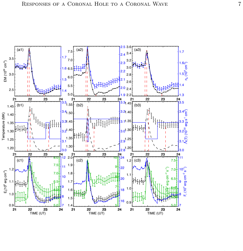
The central diagnostic is differential emission measure (DEM) analysis applied to six EUV passbands from SDO/AIA, giving maps of emission measure and a DEM-weighted mean temperature over the coronal hole. The electron density is derived from n_e = $\sqrt$(EM/l) with a line-of-sight depth of l = 123 Mm, estimated from the sharp decrease of EUV intensity with height. The energy budget combines the thermal energy change E_t, radiative loss F_r based on the CHIANTI 8.0 radiative loss function, Spitzer thermal conduction F_c, and a kinetic energy flux F_k estimated from the observed density perturbation. The wave's kinematics are tracked in AIA 211 Å base-difference and ASO-S/LST 1216 Å running-difference images, and adiabatic expectations are checked by comparing observed temperature with T proportional to n_e^(gamma-1).

What would settle it

A spectroscopic observation of a similar wave-coronal-hole crossing that measures density from line ratios independent of the assumed 123 Mm depth, combined with a check for the predicted post-wave density deficit, would settle whether the reported energy input is real; the temperature rise would be falsified if an independent temperature diagnostic shows no 1.31 to 1.43 MK increase in comparable events.

Watch

Extended reading notes

Core claim

The central claim is that a fast coronal wave can measurably alter the thermodynamic state of a coronal hole it crosses, not merely reflect or damp at the boundary. The authors observe two wave components, one moving at about 950 km/s and another at about 470 km/s; the fast component traverses the coronal hole while the slow one accumulates at its boundary as a stationary-mode wave. During the wave passage, emission measure, temperature, and density all peak within 6 to 8 minutes, then decline, and about one hour later the hole shows a higher temperature and a 14 percent lower density than before. The authors attribute the changes to adiabatic compression, wave dissipation, and possibly reconnection heating, and estimate that about 70 percent of the incoming wave energy is reflected or converted at the boundary. They compute a total energy input to the coronal hole of 2.2e8 erg $cm^{-2}$, of which roughly 3.3e7 erg $cm^{-2}$ remains as dissipated wave energy after accounting for adiabatic effects.

Load-bearing premise

The density and all derived energies rest on a single assumed line-of-sight depth of 123 Mm for the coronal hole, and the DEM-weighted temperature rise is reproduced by only 80 percent of the Monte Carlo realizations, so both the density and temperature parts of the claim are sensitive to these assumptions.

Editorial extensions

If this is right

A fast coronal wave can deliver roughly 5.1e5 erg s^-1 cm^-2 into a coronal hole during a short passage, a flux comparable to the steady energy requirement for heating coronal holes or accelerating the solar wind.
The two observed wave components behave differently: the fast component crosses the coronal hole, while the slower component stalls at the boundary and forms a stationary-mode brightening.
The plasma follows an adiabatic compression curve early in the rise, then warms further, indicating that wave dissipation or reconnection heating adds energy beyond compression.
About 70 percent of the incoming wave energy is reflected or converted at the coronal hole boundary, so only a fraction of the wave's energy enters the hole.
One hour after the wave, the coronal hole reaches a new equilibrium with higher temperature and 14 percent lower density, suggesting the deposited energy drove plasma out of the open-field region.

Reading between the lines

Editorial extensions of the paper, not claims the author makes directly.

If this energy input is typical, repeated fast waves during an active region's lifetime could contribute a non-negligible share of the coronal heating budget on open-field lines, especially in coronal holes near active regions.
The post-wave density deficit implies a net mass loss from the coronal hole; a testable extension would be to search for Doppler-shifted outflow signatures in the hours following such a wave.
The temperature rise is the most fragile part of the claim, since only 80 percent of Monte Carlo realizations reproduce it; future work with spectroscopic temperature diagnostics could separate adiabatic compression from true wave dissipation.
The method of comparing observed temperature with the adiabatic T-proportional-to-n^(gamma-1) curve could be applied to other wave-coronal-hole events as a simple diagnostic for distinguishing compressional from dissipative heating.

Share X Bluesky LinkedIn Reddit HN

Editorial analysis

A structured set of objections, weighed in public.

Desk editor's note, referee report, and a circularity audit.

Desk Editor's Note

read the letter

Main take: this is a real observation of a fast wave hitting a coronal hole, and the authors did the right kind of DEM analysis. The problem is the press line: the 2.2e8 erg/cm2 quoted in the abstract and conclusion is the gross thermal-energy increase during compression, not what the wave actually deposits. The authors know this—they compute the adiabatic part separately and get 3.3e7 erg/cm2 net—but they put the gross number in the abstract without the caveat, and then compare the corresponding flux to coronal-heating and solar-wind requirements. That comparison is off by a factor of ~6.7 if you use the net number. That is a framing error, not a fabrication.

What's genuinely new: first combined AIA EUV and ASO-S/SDI Lyman-alpha observation of a wave-CH interaction, with DEM-derived temperature and density evolution before, during, and an hour after the wave. Prior work mostly tracked wave kinematics at CH boundaries; this paper actually gives a per-unit-area energy budget for the CH interior, the boundary, and the body separately. The adiabatic curve check in Fig. 5 is a nice touch—it shows the early rise is compression, and the subsequent deviation is where real dissipation might be happening. That is honest and useful.

Soft spots, in order of importance. First, the gross/net issue above. Second, the LOS depth l=123 Mm is set from a sharp EUV intensity drop, but no error is assigned; n_e scales as l^{-1/2}, so the energy numbers shift, but the temperature and density comparisons don't. Third, the authors note only 80% of Monte Carlo realizations show the temperature rise; that makes the T increase fragile, and the abstract states it without this caveat. The 14% density decrease is more robust because it comes from EM. Fourth, the radiative and conduction terms use standard formulas but with rough geometry; those are at the 10^6 level while the headline is 10^8, so they aren't the main issue.

Who is this for: solar physicists working on EUV waves, coronal holes, and wave-energy deposition. It is a case study, not a population study, so it won't settle the solar wind heating question. But it gives a concrete number and a method. It deserves referee time, though the authors should be asked to either lead with the net number or clearly separate the transient compression energy from the dissipated energy, and to add a sensitivity test on l. The qualitative result—transient EM rise then a persistent density drop—probably holds.

Referee Report

3 major / 6 minor

Summary. The paper reports observations of an X5.0 flare-driven coronal wave on 2023 December 31, detected simultaneously in SDO/AIA EUV images and ASO-S/LST Lyman-alpha images, and studies its interaction with an adjacent coronal hole. Using DEM analysis, the authors find that during the wave passage the coronal hole's DEM-weighted temperature increased from 1.31 to 1.43 MK and its electron density from about 1.62e8 to 1.76e8 cm^-3 over a ~7-minute rising phase, followed by a new quasi-equilibrium state with a slight temperature increase and a 14% density decrease. They estimate the energy input from the wave as ΔE = ΔE_t + ΔE_r + ΔE_c = 2.2±0.3e8 erg cm^-2 and compare the corresponding average flux of 5.1e5 erg s^-1 cm^-2 with coronal heating and solar wind energy requirements. The paper also separates the fast (~950 km/s) and slow (~470 km/s) wave components and discusses wave reflection and mode conversion at the coronal hole boundary.

Significance. If the central energy claim were supportable, this would be a valuable quantitative measurement of how a fast coronal wave transfers energy into an open-field region, with implications for coronal heating and solar wind acceleration. The paper's strengths include the multi-instrument identification of the wave in both EUV and Lyman-alpha, the use of DEM to track temperature and emission measure, explicit Monte Carlo uncertainty propagation for the DEM-derived quantities, and a three-region decomposition (whole CH, boundary, main body) that attempts to separate boundary effects. The adiabatic comparison in Section 2.3 is also a useful diagnostic. However, as discussed in the major comments, the headline energy figure is a gross internal-energy change rather than a net dissipated energy, and the authors' own adiabatic subtraction reduces the latter by a factor of about 6.7. This, together with the sensitivity of the results to the assumed line-of-sight depth and the modest statistical robustness of the temperature increase, means the paper's most prominent claims need substantial revision before publication.

major comments (3)

[Abstract; Section 2.3, ΔE = ΔE_t + ΔE_r + ΔE_c; Section 3, first two paragraphs] The headline energy of 2.2±0.3e8 erg cm^-2 is the change in thermal energy during the rising phase, but the authors themselves show in Section 2.3 that the observed temperature closely follows the adiabatic curve T/n^(γ-1)=constant and that the adiabatic contribution to the thermal-energy increase is 1.8e8 erg cm^-2. After subtracting adiabatic compression and the small radiative and conductive losses, their own calculation leaves only 3.3e7 erg cm^-2 as energy dissipated into the CH. Adiabatic compression is reversible, so the abstract's statement that the wave 'provided' 2.2e8 erg cm^-2 and the conclusion's comparison of 5.1e5 erg s^-1 cm^-2 to coronal heating/solar wind requirements are not supported by the net energy deposition. The net value, 3.3e7 erg cm^-2 over ~430 s, corresponds to ~7.7e4 erg s^-1 cm^-2, an order of magnitude smaller. The manuscript should either reframe the headline as a gross transient internal-energy change with the adiabatic part clearly labeled as reversible, or make the net dissipated energy the central quantity.
[Section 2.2, ne = sqrt(EM/l) and 'considered as 123 Mm'] The line-of-sight depth l=123 Mm is a single hand-set value that enters directly into ne=sqrt(EM/l), Et=(3/2)2ne kT l, Fr=ne^2 Λ(T)l, and Fc≈-(2/7)κT^{7/2}/l. The justification given, 'sharp decrease in EUV intensity above this height over the east of the CH,' is not documented with the actual intensity profile or an uncertainty estimate. If the emitting depth differs by, say, a factor of two, the derived density and thermal-energy changes, and therefore the energy budget, change significantly. Please provide the supporting intensity-height profile, a systematic uncertainty estimate for l, or a sensitivity analysis showing how the final energy input and the net dissipated energy vary with l.
[Section 3, final paragraph; Figure 5(b1-b3)] The temperature increase is a load-bearing part of the energy calculation, since ΔE_t dominates the budget, yet the authors report that only 80% of the Monte Carlo realizations from the DEM method show the increase. This means the 1.31→1.43 MK rise is not robust at the 95% level, and the black unavailable region in Figure 4(h) indicates data-quality issues in part of the CH. The manuscript should quantify how the energy budget changes when only realizations that do show the temperature increase are used, and should state explicitly in the abstract and conclusions that the temperature part of the result has this fragility. Without that caveat, the confidence conveyed by 'increase in temperature from 1.31 to 1.43 MK' is misleading.

minor comments (6)

[Title and text throughout] There are numerous typographical errors, including 'F ast' and 'W ave' in the title, 'trasmited', 'Atronomical', 'mintues', 's1-s2' versus 'S1-S2' in Section 2.1, and '21 ˚A' for what should be '211 ˚A'. A thorough language and proofreading pass is needed.
[Figure 1 caption and panel references] The caption lists panels (a)-(f), but the text refers to 'Panel (g)' for the GOES soft X-ray flux. Either add the panel or correct the reference.
[Section 2.1, 'Zhou et al. (2025, in preparation)'] Citing a paper 'in preparation' for the first Lyman-alpha coronal wave identification is not ideal; please replace with a published reference or clearly mark it as a personal communication and remove it from the reference list.
[Section 2.3, conduction flux formula] The sentence 'Assuming force-free fields' to justify the Spitzer conduction formula is confusing; thermal conduction is along the magnetic field regardless of whether the field is force-free. Rephrase to say 'assuming the temperature gradient is along the magnetic field over a length scale l' or similar.
[Section 2.2, DEM temperature definition] The formula for the DEM-weighted temperature T̄ is written inline and is hard to parse; please display it as an equation and specify whether the logarithm is base 10 or natural logarithm when giving the integration range [5.4, 6.9].
[Figure 5] The panel labels (a1-a3, b1-b3, c1-c3) are not all consistently described in the caption, and the caption for panel (a2-c2) says 'CH area' while the text lists three regions. Please clarify which panel corresponds to which region in the caption.

Circularity Check

0 steps flagged · score 0.0 of 10

No significant circularity: the energy budget is an accounting of measured DEM-derived plasma parameters using standard formulas, and the adiabatic/dissipation decomposition is openly stated and quantified.

full rationale

The paper's central quantitative claims (temperature/density changes and the 2.2e8 erg cm^-2 energy input) are derived directly from DEM measurements and standard formulas: n_e = sqrt(EM/l), E_t = 3 n_e k T l, F_r = EM Lambda(T), and F_c = -(2/7) kappa T^(7/2)/l. None of these parameters are fitted to reproduce the headline energy; the DEM inversion (Cheung et al. 2015) is external and standard, and the line-of-sight depth of 123 Mm is an observed assumption stated in the text. The claim that adiabatic compression accounts for 1.8e8 erg cm^-2 of the thermal increase is explicitly presented as a model-based subtraction, and the paper itself reports the residual dissipated energy as 3.3e7 erg cm^-2, so there is no hidden equivalence between input and output. The only self-referential citation (Zhou et al. 2025, in preparation, for Lyman-alpha wave detection) is not load-bearing: the Lyman-alpha wave is directly observed in the paper's own running-difference images. The paper also discloses the fragility of the temperature increase (80% of Monte Carlo realizations) and the assumption of constant mass/energy injection from the chromosphere; these are limitations that affect robustness, not circularity. The derivation chain is self-contained against observational data and external standard formulas, so no circular step is identified.

Assumptions & free parameters 3 free parameters · 6 assumptions · 0 invented entities

The central calculation is an energy accounting built from observed EM and T maps, not a closed-form derivation. The main 'pulled from upstream' items are the standard DEM method, CHIANTI radiative losses, and Spitzer conduction; none is circular. The most fragile input is the hand-set LOS depth of 123 Mm and the chosen DEM temperature range, which scale the headline numbers. There are no invented particles, forces, or fields.

free parameters (3)

Line-of-sight depth of CH = 123 Mm
Adopted from 'sharp decrease in EUV intensity above this height' (Section 2.2). It enters n_e = sqrt(EM/l), thermal energy, and conduction terms, so the reported density and energy budget depend on it.
DEM integration temperature range = log T in [5.4, 6.9]
Used to define DEM-weighted mean temperature T (Section 2.2). The choice affects all temperatures, radiative losses, and conduction fluxes, and is not varied in a reported sensitivity test.
Rising period for time integration = ~7 minutes (430 s)
Chosen from the EM/T profiles for energy integration. The time-integrated losses and kinetic energy scale linearly with this window.

assumptions (6)

domain assumption AIA DEM inversion of optically thin, collisionally excited plasma yields unbiased EM and T in the coronal hole.
Used through Cheung et al. (2015) DEM method (Section 2.2). Coronal holes are low-emission regions, so background and foreground contamination can bias results; no independent calibration is given.
ad hoc to paper The coronal hole has a constant line-of-sight emitting depth of 123 Mm.
Justified in Section 2.2 only by a qualitative statement about EUV intensity decrease above this height; no measurement or model is cited. This is load-bearing for n_e and energy.
domain assumption The plasma is fully ionized and dominated by hydrogen, with total particle density 2 n_e.
Used in E_t = 3 n_e k T l (Section 2.3). Departures change the thermal energy estimate.
domain assumption Heat conduction follows the Spitzer law with a linearized gradient giving F_c = -(2/7) kappa T^(7/2)/l in a force-free field.
Section 2.3 uses this approximation because the true temperature gradient along the field is not observed.
standard math Compression and expansion are adiabatic with gamma = 5/3.
Section 2.3 uses T/n^(gamma-1) = constant to separate adiabatic and dissipative contributions.
domain assumption Velocity perturbation obeys delta v / v_ph >= delta rho / rho, giving a lower bound on kinetic energy flux.
Section 2.3 uses this to estimate F_k and E_k from density changes only, without measuring wave velocities directly.

how reviews work

0 comments

Cite this review

Pith. "Pith review of Responses of a Coronal Hole to a Fast Flare-Driven Coronal Wave." pith.science (2026). https://pith.science/paper/GOUSZ5DB

@misc{pith2026250608863,
  author       = {Pith},
  title        = {Pith review of: Responses of a Coronal Hole to a Fast Flare-Driven Coronal Wave},
  year         = {2026},
  howpublished = {\url{https://pith.science/paper/GOUSZ5DB}},
  note         = {Machine review of arXiv:2506.08863}
}

abstract

Coronal waves, significant solar phenomena, act as diagnostic tools for scientists studying solar atmosphere properties. Here, we present a novel observation detailing how a coronal wave event, associated with an X5.0 class flare, influenced the properties of an adjacent coronal hole through interaction. The coronal wave was observed in both extreme ultraviolet observations from the Atmospheric Imaging Assembly aboard the Solar Dynamics Observatory and Lyman-alpha observations from the Solar Disk Imager aboard the Advanced Space-based Solar Observatory. Utilizing the method of differential emission measure, we found that as the coronal wave passed through, the adjacent coronal hole experienced an increase in temperature from 1.31 to 1.43 MK and a rise in density from $\sim$1.62$\times10^{8}$ to 1.76$\times10^{8}$ cm$^{-3}$ within the rising period of $\sim$7 minutes. Subsequently, after the wave passed, the entire coronal hole transitioned to a new state with a slight temperature increase and a 14$\%$ decrease in density, with more pronounced changes observed at the coronal hole's boundary. Taking into account the impacts of radiative loss and heat conduction, the coronal wave was estimated to provide an average energy of 2.2$\times10^{8}$ erg cm$^{-2}$ to the coronal hole during the short rising period. This study highlights the identification of the coronal wave in both extreme ultraviolet and Lyman-alpha observations, shedding light on the significant energy input, particularly within the coronal hole. These findings provide new insights into better understanding kinematics of fast coronal waves, energy transfer processes open versus closed magnetic topologies, and the possible acceleration of solar winds.

Figures

Figures reproduced from arXiv: 2506.08863 by the authors.

**Figure 1.** Multi-wavelength observations revealing the flare-associated coronal wave and its sweeping region. Panel (a) displays an HMI image at 20:58 UT on December 31, showcasing AR13536 in N05E75, a nearby polarity inversion line (PIL) indicated by a white dashed line, and the examined CH with predominantly positive polarity outlined by yellow contours. In Panel (b), an image at 1216 ˚A from the LST illustrates the flare pr… view at source ↗

**Figure 2.** The coronal wave is evident in the running difference UV images at 1216 ˚A (top row) and the base difference EUV images at 211 ˚A (bottom two rows). The advancing fronts of the wave are delineated by white curves in Panels (a-b) and appear as white features in the bottom two rows. Notably, the wave exhibited an accumulation at the boundary of the CH, as indicated by the green contour in Panel (f). The CH is outlined… view at source ↗

**Figure 3.** Two types of coronal waves illustrated in the time-distance maps along the slice “S1-S2” as depicted in [PITH_FULL_IMAGE:figures/full_fig_p005_3.png] view at source ↗

Figures from the paper (2 more)

**Figure 4.** Figure 4: Evolution and distribution of emission measure (EM) and temperature (T) within the CH delineated by black contours. The EM and T within the CH were estimated by DEM analysis using AIA data from six wavelengths: 131, 171, 193, 21, 335, and 94 ˚A. Panel (a) and (e) displ…

**Figure 5.** Figure 5: Time profiles of essential parameters were analyzed to understand the dynamics within the CH. In Panels (a1-a2), the evolution of EM (black curves), electron number density (ne, blue curves) with 1σ uncertainties are depicted. Panels (b1-b2) display the DEM-weighted me…

Discussion (0). Sign in to comment.

Reference graph

Works this paper leans on

57 extracted references · 57 canonical work pages

[1]

J.\ 2004, SOHO 15 Coronal Heating, 575, 97

Aschwanden, M. J.\ 2004, SOHO 15 Coronal Heating, 575, 97

work page 2004
[2]

F., Wu, S

Chen, P. F., Wu, S. T., Shibata, K., et al.\ 2002, , 572, L99

work page 2002
[3]

F.\ 2011, LRSP, 8, 1

Chen, P. F.\ 2011, LRSP, 8, 1

work page 2011
[4]

F., Fang, C., Chandra, R., et al.\ 2016, , 291, 3195

Chen, P. F., Fang, C., Chandra, R., et al.\ 2016, , 291, 3195

work page 2016
[5]

Chen, B., Li, H., Song, K.-F., et al.\ 2019, RAA, 19, 159

work page 2019
[6]

Chen, H., Fletcher, L., Zhou, G., et al.\ 2024, , 976, 207

work page 2024
[7]

Cheung, M. C. M., Boerner, P., Schrijver, C. J., et al.\ 2015, , 807, 143

work page 2015
[8]

P., Young, P

Del Zanna, G., Dere, K. P., Young, P. R., et al.\ 2021, , 909, 38

work page 2021

Show all 57 references

[9]

I., van der Holst, B., et al.\ 2012, , 750, 2, 134

Downs, C., Roussev, I. I., van der Holst, B., et al.\ 2012, , 750, 2, 134

2012
[10]

Feng, L., Li, H., Chen, B., et al.\ 2019, RAA, 19, 162

2019
[11]

R., Hudson, H

Fletcher, L., Dennis, B. R., Hudson, H. S., et al.\ 2011, , 159, 19

2011
[12]

T., Mathioudakis, M., Keenan, F

Gallagher, P. T., Mathioudakis, M., Keenan, F. P., et al.\ 1999, , 524, L133

1999
[13]

Gan, W.-Q., Zhu, C., Deng, Y.-Y., et al.\ 2019, RAA, 19, 156

2019
[14]

Gopalswamy, N., Yashiro, S., Temmer, M., et al.\ 2009, , 691, 2, L123

2009
[15]

Hannah, I. G. & Kontar, E. P.\ 2012, , 539, A146

2012
[16]

Hou, Z., Tian, H., Wang, J.-S., et al.\ 2022, , 928, 98

2022
[17]

Huber, M. C. E., Foukal, P. V., Noyes, R. W., et al.\ 1974, , 194, L115

1974
[18]

W., Veronig, A

Kienreich, I. W., Veronig, A. M., Muhr, N., et al.\ 2011, , 727, L43

2011
[19]

A., Korreck, K

Kozarev, K. A., Korreck, K. E., Lobzin, V. V., et al.\ 2011, , 733, L25

2011
[20]

R., Title, A

Lemen, J. R., Title, A. M., Akin, D. J., et al.\ 2012, , 275, 17

2012
[21]

Li, H., Chen, B., Feng, L., et al.\ 2019, RAA, 19, 158

2019
[22]

Li, C., Fang, C., Li, Z., et al.\ 2019, RAA 19, 165

2019
[23]

Li, C., Fang, C., Li, Z., et al.\ 2022, SCPMA, 65, 289602

2022
[24]

M., Zhao, J., et al.\ 2011, , 736, L13

Liu, W., Title, A. M., Zhao, J., et al.\ 2011, , 736, L13

2011
[25]

V., et al.\ 2012, , 753, 52

Liu, W., Ofman, L., Nitta, N. V., et al.\ 2012, , 753, 52

2012
[26]

& Ofman, L.\ 2014, , 289, 9, 3233

Liu, W. & Ofman, L.\ 2014, , 289, 9, 3233

2014
[27]

Liu, W., Jin, M., Downs, C., et al.\ 2018, , 864, 2, L24

2018
[28]

Liu, Q., Tao, H., Chen, C., et al.\ 2022, SCPMA, 65, 289605

2022
[29]

M., Gallagher, P

Long, D. M., Gallagher, P. T., McAteer, R. T. J., et al.\ 2008, , 680, L81

2008
[30]

Munro, R. H. & Withbroe, G. L.\ 1972, , 176, 511

1972
[31]

V., Schrijver, C

Nitta, N. V., Schrijver, C. J., Title, A. M., et al.\ 2013, , 776, 58

2013
[32]

Olmedo, O., Vourlidas, A., Zhang, J., et al.\ 2012, , 756, 143

2012
[33]

D., Thompson, B

Pesnell, W. D., Thompson, B. J., & Chamberlin, P. C.\ 2012, , 275, 3

2012
[34]

Piantschitsch, I., Vr s nak, B., Hanslmeier, A., et al.\ 2018, , 860, 1, 24

2018
[35]

Piantschitsch, I., Terradas, J., Soubrie, E., et al.\ 2024, , 687, A200

2024
[36]

Priest, E.\ 2014, Magnetohydrodynamics of the Sun, by Eric Priest, Cambridge, UK: Cambridge University Press, 2014

2014
[37]

Qiu, Y., Rao, S., Li, C., et al.\ 2022, SCPMA, 65, 289603

2022
[38]

& Vaiana, G

Rosner, R. & Vaiana, G. S.\ 1977, , 216, 141

1977
[39]

F., Massa, P., Battaglia, A

Ryan, D. F., Massa, P., Battaglia, A. F., et al.\ 2024, , 299, 114

2024
[40]

H., Schou, J., Bush, R

Scherrer, P. H., Schou, J., Bush, R. I., et al.\ 2012, , 275, 207

2012
[41]

Schmidt, J. M. & Ofman, L.\ 2010, , 713, 2, 1008

2010
[42]

M., Holman, G

Su, Y., Veronig, A. M., Holman, G. D., et al.\ 2013, NatPh, 9, 489

2013
[43]

Su, Y., Liu, W., Li, Y.-P., et al.\ 2019, RAA, 19, 163

2019
[44]

M., Dissauer, K., et al.\ 2015, , 812, 173

Vanninathan, K., Veronig, A. M., Dissauer, K., et al.\ 2015, , 812, 173

2015
[45]

M., Temmer, M., & Vr s nak, B.\ 2008, , 681, L113

Veronig, A. M., Temmer, M., & Vr s nak, B.\ 2008, , 681, L113

2008
[46]

M., Podladchikova, T., Dissauer, K., et al.\ 2018, , 868, 107

Veronig, A. M., Podladchikova, T., Dissauer, K., et al.\ 2018, , 868, 107

2018
[47]

Wang, C., Chen, F., & Ding, M.\ 2021, , 911, L8

2021
[48]

Warmuth, A.\ 2015, LRSP, 12, 3

2015
[49]

Withbroe, G. L. & Noyes, R. W.\ 1977, , 15, 363

1977
[50]

L.\ 1988, , 325, 442

Withbroe, G. L.\ 1988, , 325, 442

1988
[51]

Zhang, Z., Chen, D.-Y., Wu, J., et al.\ 2019, RAA, 19, 160

2019
[52]

M., Cheng, J

Zhang, Q. M., Cheng, J. X., Feng, L., et al.\ 2019, , 883, 124

2019
[53]

Zheng, R., Chen, Y., Feng, S., et al.\ 2018, , 858, L1

2018
[54]

Zheng, R.\ 2024, RSPSA, 480, 20230950

2024
[55]

Zhou, G., Gao, G., Wang, J., et al.\ 2020, , 905, 150

2020
[56]

Zhou, X., Shen, Y., Tang, Z., et al.\ 2022, , 659, A164

2022
[57]

Zhou, X., Shen, Y., Yuan, D., et al.\ 2024, NatCo, 15, 3281

2024

Pith tools

Reviewed August 7, 2026 · model on record in the stance chip above.

[1] [1]

J.\ 2004, SOHO 15 Coronal Heating, 575, 97

Aschwanden, M. J.\ 2004, SOHO 15 Coronal Heating, 575, 97

work page 2004

[2] [2]

F., Wu, S

Chen, P. F., Wu, S. T., Shibata, K., et al.\ 2002, , 572, L99

work page 2002

[3] [3]

F.\ 2011, LRSP, 8, 1

Chen, P. F.\ 2011, LRSP, 8, 1

work page 2011

[4] [4]

F., Fang, C., Chandra, R., et al.\ 2016, , 291, 3195

Chen, P. F., Fang, C., Chandra, R., et al.\ 2016, , 291, 3195

work page 2016

[5] [5]

Chen, B., Li, H., Song, K.-F., et al.\ 2019, RAA, 19, 159

work page 2019

[6] [6]

Chen, H., Fletcher, L., Zhou, G., et al.\ 2024, , 976, 207

work page 2024

[7] [7]

Cheung, M. C. M., Boerner, P., Schrijver, C. J., et al.\ 2015, , 807, 143

work page 2015

[8] [8]

P., Young, P

Del Zanna, G., Dere, K. P., Young, P. R., et al.\ 2021, , 909, 38

work page 2021