REVIEW 4 major objections 5 minor 52 references
Observations of Carbon Radio Recombination Lines with the NenuFAR telescope. I. Cassiopeia A and Cygnus A
T0 review · 4 major / 5 minor · reviewed 2026-08-07 · deepseek-v4-flash
Pith's one-line read NenuFAR observations of Cassiopeia A and Cygnus A yield 398 carbon radio recombination lines and, from their quantum-number-dependent shapes, electron temperatures about 50% lower, densities about 35% lower, and turbulent velocities…
desk verdict NenuFAR's first CRRL paper is a solid instrument validation with real detections and a genuine sensitivity gain, but the claimed quantitative differences from LOFAR are not yet robust because the fitted line intensities are never corrected for the beam dilution the paper itself documents. read the letter →
The pith
A machine-rendered reading of the paper's core claim, the machinery that carries it, and where it could break.
The reading
What carries the argument
The central object is the carbon radio recombination line: a transition between adjacent high Rydberg levels ($n+1$ to $n$, here $n=426$ to $826$) seen in absorption against a bright background source at 10 to 85 MHz. Each stacked line is decomposed into a Voigt profile, whose Gaussian (Doppler) width carries the electron temperature $T_e$ and the mean turbulent velocity $v_t$, whose Lorentzian width carries pressure, natural, and radiation broadening set by $T_e$, $n_e$, and the radiation field temperature $T_0$, and whose integrated area carries $T_e$, $n_e$, and cloud length $L$ through departure coefficients. The machinery works because these contributions scale differently with principal quantum number $n$, so the $n$-dependence of the linewidths and integrated areas separates the five physical parameters from a single set of absorption spectra.
What would settle it
Image Cas A and Cygnus A with an interferometer that can synthesize beams from about 5 arcminutes to 3.6 degrees at the same frequencies, and measure the integrated C$\alpha$ line-to-continuum ratio as a function of beam diameter: if the ratio falls as the beam grows, the dilution-by-diffuse-background explanation is confirmed, while if the ratio is beam-independent, the offset instead comes from calibration or from the fitting priors such as the $n>560$ area constraints.
Extended reading notes
Core claim
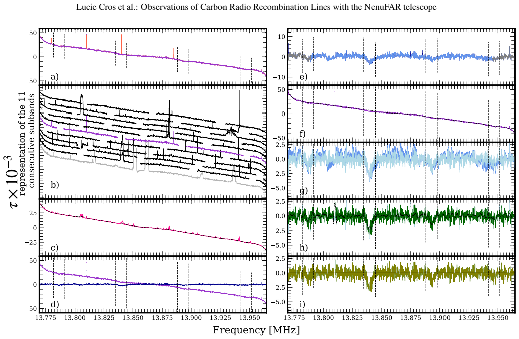
Using 71.5 hours on Cassiopeia A and 157.5 hours on Cygnus A in NenuFAR beamforming mode at 95.4 Hz spectral resolution, the authors detect 398 individual C$\alpha$ absorption lines toward Cas A between principal quantum numbers $n=426$ and $n=826$, and obtain eleven usable stacked detections toward Cyg A. They fit Voigt profiles to stacks of 7 to 50 transitions and extract linewidth and integrated line-to-continuum intensity as functions of $n$. Fitting the $n$-dependence with the recombination model of Salgado et al. (2017a,b), they find for the Cas A clouds at $-47$, $-38$, and $0$ km/s respectively: $T_e=45$, $40$, and $52$ K; $n_e=0.027$, $0.025$, and $0.014$ cm$^{-3}$; $v_t=3.3$, $4.7$, and $3.7$ km/s. For the Cygnus A cloud at $3.5$ km/s they find $T_e=77$ K, $n_e=0.018$ cm$^{-3}$, and $v_t=7.9$ km/s. These values imply thermal pressures of a few times $10^3$ K cm$^{-3}$, dominated by turbulent pressure, consistent with standard interstellar medium models. Compared with LOFAR-based estimates for the same sightlines, the NenuFAR fits are on average about 50 percent cooler, about 35 percent less dense, and 10 to 80 percent more turbulent, an offset the paper attributes to NenuFAR's larger beam and the resulting dilution of the line-to-continuum ratio.
Load-bearing premise
The modeling treats each detected velocity component as a single uniform cloud with one electron density and one temperature along the line of sight, seen against an unresolved point-like background; the paper's own comparison shows that line intensities toward Cas A differ by tens of percent between LOFAR and NenuFAR, indicating that this beam-independence condition may not hold and that the fitted $n_e$ and $T_e$ could be biased by dilution.
Editorial extensions
If this is right
- NenuFAR can routinely detect carbon radio recombination lines across 10–85 MHz: 398 individual C$\alpha$ lines toward Cassiopeia A and usable stacked lines toward Cygnus A, with signal-to-noise about four times higher than LOFAR at matched resolution and about ten times higher when identical transitions are stacked.
- Resolving three separate velocity components toward Cas A, including the faint 0 km/s component, shows that the new telescope can measure cloud-by-cloud physical conditions rather than a single blended average.
- The derived pressures, with thermal pressure a few thousand K cm$^{-3}$ and turbulent pressure dominating in all four clouds, match standard expectations for the diffuse neutral interstellar medium, indicating that the fitting procedure returns physically plausible results.
- If the beam-size interpretation is correct, low-frequency CRRL absorption depends not only on the foreground clouds but also on the beam's overlap with the resolved Galactic background, so future surveys must model beam dilution explicitly when comparing instruments.
- The $n$-dependence of line shape can now be measured over a wider quantum-number range than before, which sharpens the constraints on where the Doppler-dominated regime transitions to the Lorentzian-dominated regime around $n=580$.
Reading between the lines
- If beam dilution is real, earlier LOFAR absorption measurements toward Cas A likely mix true cloud physics with the fraction of background continuum inside the beam, so published $n_e$ and $T_e$ values for these sightlines may need downward revision by tens of percent, and not only for NenuFAR comparisons.
- Because NenuFAR's beam reaches 3.6 degrees at 10 MHz, the same technique could turn CRRL absorption from a source-by-source probe into a tomographic survey of the diffuse interstellar medium across large areas of the Galactic plane, using many background sources rather than the two brightest ones.
- The paper reports poor constraints on $T_0$ and $L$ and a multimodal parameter space; a natural extension would be joint fitting of CRRL line shapes with independent tracers such as HI 21-cm absorption, CO, or dust extinction along the same sightlines, which could fix the cloud length and radiation field separately and break the degeneracy.
- The smaller LOFAR-NenuFAR discrepancy toward the high-latitude Cygnus A sightline than toward the low-latitude Cas A sightline suggests that the diffuse Galactic background itself contributes to CRRL absorption, implying a testable prediction: CRRL optical depth toward extragalactic sources should increase as the telescope beam encompasses more Galactic plane.
Editorial analysis
A structured set of objections, weighed in public.
Referee Report
Summary. The paper presents NenuFAR observations of carbon radio recombination lines in absorption towards Cassiopeia A and Cygnus A. After developing a substantial RFI-mitigation and baseline-correction pipeline, the authors detect 398 C-alpha lines toward Cas A between principal quantum numbers n=426 and n=826, stack them into 28 groups, and fit Voigt profiles to three foreground velocity components. For Cyg A they obtain 11 stacked detections toward one component. From the fitted integrated line-to-continuum intensities and line widths (Appendix B), a five-parameter grid search yields electron temperatures, densities, radiation-field temperatures, cloud sizes, and turbulent velocities. The headline result is that the NenuFAR-derived T_e is roughly 50% lower, n_e roughly 35% lower, and v_t 10\u201380% higher than previous LOFAR-based estimates, which the authors attribute to the larger NenuFAR beam sampling a larger volume of diffuse gas.
Significance. If the parameter extraction were robust, this paper would be a significant demonstration that a large single-dish beam can recover CRRL absorption spectra with very high signal-to-noise, and that low-frequency CRRL line shapes are sensitive to the spatial scale of the sampled ISM. The manuscript is honest about many limitations, presents a detailed pipeline, compares directly with LOFAR spectra, and makes the stacked spectra and fitted line parameters available in tables. However, the central quantitative claim\u2014the comparison of T_e, n_e, and v_t with LOFAR\u2014is currently not supported because the forward model omits the beam-dilution effect that the paper itself identifies, and because the fits in the regime that matters most have reduced chi-square values far above one. The paper would be a useful technical and observational benchmark even if the astrophysical comparison were reframed as preliminary.
major comments (4)
- [Section 5.1, Eq. (B.4), Fig. 14] The forward model for the integrated line-to-continuum intensity, Eq. (B.4), contains no covering factor or beam-dilution term. The observed A_n is the integral of I_line/I_cont over frequency, so any foreground or background continuum that is not intercepted by the absorbing cloud will multiply the measured A_n by a frequency-dependent factor below unity. The paper's own Fig. 14 shows A_NenuFAR/A_LOFAR dropping to roughly 0.6\u20130.8 at low frequencies toward Cas A, which Sect. 5.1 attributes to dilution by a resolved Galactic background. Because A_n enters the chi-square statistic (Eq. B.16) and scales as n_e^2 T_e^-2.5, an uncorrected 20\u201340% suppression can shift the inferred n_e and T_e at approximately the level of the claimed LOFAR differences. Moreover, the direction of the shift is not trivial: lower observed A_n at fixed T_e would bias n_e downward, but the paper also derives T_e lower than LOFAR, which would increase A_n and require an even larger dilution factor. The paper must either include a dilution/covering-factor parameter in the forward model, calibrate A_n against an external absolute scale, or explicitly restrict the quantitative LOFAR comparison to the high-frequency regime where the dilution is small.
- [Section 4.1.2] For n above 560, the fitting procedure imposes hard priors that force the line area of the \u221238 km s^-1 component to be at most one third of the \u221247 km s^-1 area, and the 0 km s^-1 area to be no larger than the \u221238 km s^-1 area. These priors are introduced specifically to manage blending, but they are applied exactly in the regime where the model later fails to reproduce the data (Sect. 4.1.3). The physical parameters reported in Table 2 therefore are not determined from the data alone in this part of the spectrum. The authors should demonstrate that the fitted parameters are robust to relaxing these priors, for example by repeating the fit on a subset of stacks or by leaving the area ratios free with weak logarithmic priors and checking that the results are stable.
- [Section 4.1.3, Appendix D] The quoted best fits have reduced chi-square values of about 6.7 for the \u221247 km s^-1 component and 5.3 for the \u221238 km s^-1 component (Figs. D.1 and D.2), while the reported uncertainties are simply the parameter sets within 30% of the optimal chi-square. With chi-square_r >> 1, those uncertainty envelopes and the central values themselves are not statistically meaningful, and the model does not reproduce the observed line-width and intensity curves. This is particularly serious because the paper's LOFAR comparison relies on the exact values of T_e and n_e. The authors should either improve the model (e.g., multi-component or non-uniform clouds) or present the parameter estimates as indicative rather than as measured values.
- [Section 4.1.3, Eq. (B.16)] The text states that for n greater than about 600 the measured integrated line-to-continuum intensity collapses because of blending and is not physical, and that the effect 'should not impact the optimisation process.' However, the chi-square definition in Eq. (B.16) includes all stacks used in the analysis, and the grid search presumably uses the same A_n values shown in Fig. 8. If the n>600 points are not excluded from the fit, the optimization is pulled by exactly the regime the authors say cannot be modeled. The manuscript must state clearly whether those points are included or excluded, and, if included, must justify their use despite the acknowledged model failure.
minor comments (5)
- [Abstract] The symbol '3 t' appears in the abstract and elsewhere; this should be the mean turbulent velocity v_t (or \sigma_t) with proper mathematical formatting.
- [Conclusion] The first cloud toward Cas A is quoted with T_0 = 1200 K in the concluding remarks, while Section 4.1.3 and Table 2 give T_0 = (1700 \u00b1 100) K. Please correct the inconsistency.
- [Fig. D.3 caption] The caption labels the panel as 'Cassiopeia A, component \u221247 km s^-1', but the text and panel headers refer to the 0 km s^-1 component; the caption should be corrected.
- [Sections 4.1.2 and C.2] The cross-reference 'Table??' appears twice and should point to the actual tables of measured line properties.
- [Section 5.1] The discussion of grating lobes is qualitative. Since the authors argue the effect is negligible, a quantitative estimate (e.g., expected source confusion level or a gain pattern calculation) would be more convincing.
Circularity Check
No circularity found: the physical-parameter derivation is a standard forward-model fit to measured line shapes; the LOFAR-derived priors are not load-bearing for the central Te/ne/vt constraints.
full rationale
The paper's derivation chain runs from calibrated NenuFAR optical-depth spectra, through Voigt-profile fits of stacked C-alpha lines, to measured integrated line-to-continuum areas A_n and profile widths w_V, and finally to a chi-squared grid search over (T_e, n_e, T_0, v_t, L) using the explicit forward equations B.4-B.10. This is ordinary model fitting, not a self-referential derivation: T_e and n_e are not defined in terms of the fitted A_n and w_V; they are independent grid parameters whose model predictions are compared with the data. The LOFAR-based cloud velocities are used only as line-center priors for masking and deblending (Sect. 3.1.2), and the paper explicitly labels the need for such priors a 'significant caveat'; the line widths and areas that carry the physical constraints remain free fit outputs. The missing beam-dilution term in Eq. B.4, acknowledged in Sect. 5.1, is a potential systematic bias in the inferred T_e and n_e, but it does not make the inference equal to its inputs; an incomplete forward model is a correctness issue, not circularity. Finally, the modeling framework of Salgado et al. (2017a,b) is cited as external support, but the key equations are reproduced in Appendix B, so the derivation is self-contained; no uniqueness theorem or author-specific ansatz is invoked to force the parameter choice. The paper therefore contains no step that is equivalent by construction to its own inputs.
Assumptions & free parameters
free parameters (7)
- Electron temperature T_e =
45 K (-47), 40 K (-38), 52 K (0) for Cas A; 77 K for Cyg A
- Electron density n_e =
2.7e-2 cm^-3 (-47), 2.5e-2 (-38), 1.4e-2 (0), 1.8e-2 (Cyg A)
- Radiation field temperature T_0 =
1700 K (-47), 1200 K (-38), 1000 K (0), 1600 K (Cyg A)
- Cloud depth L =
33.0 pc (-47), 20.5 pc (-38), 15.0 pc (0), 8.0 pc (Cyg A)
- Mean turbulent velocity v_t =
3.3 km/s (-47), 4.7 (-38), 3.7 (0), 7.9 (Cyg A)
- Radiation field spectral index alpha =
-2.6 (assumed)
- S/N cap for stacking weights =
6
assumptions (6)
- domain assumption CRRL line formation model of Salgado et al. (2017a,b): departure coefficients b_n and stimulated emission factors beta_n,n' are tabulated and correct for the CNM conditions
- domain assumption Carbon is the dominant electron provider and n_CII ~ n_e in the absorbing clouds
- domain assumption Each velocity component is a single homogeneous cloud with constant T_e, n_e, and v_t along the line of sight
- domain assumption The background source is unresolved and the covering factor is unity for the absorbing clouds
- ad hoc to paper Expected line velocities and the existence of the clouds are taken from previous LOFAR studies
- standard math Voigt profile with independent Gaussian (Doppler) and Lorentzian (radiative plus pressure) widths is the correct line shape
Cite this review
Pith. "Pith review of Observations of Carbon Radio Recombination Lines with the NenuFAR telescope. I. Cassiopeia A and Cygnus A." pith.science (2026). https://pith.science/paper/3OL6K3RQ
@misc{pith2026250608895,
  author       = {Pith},
  title        = {Pith review of: Observations of Carbon Radio Recombination Lines with the NenuFAR telescope. I. Cassiopeia A and Cygnus A},
  year         = {2026},
  howpublished = {\url{https://pith.science/paper/3OL6K3RQ}},
  note         = {Machine review of arXiv:2506.08895}
}
read the original abstract
Carbon Radio Recombination Lines (CRRLs) at decametre wavelengths trace the diffuse phase of the interstellar medium (ISM) of the Galaxy. Their observation allows to measure physical parameters of this phase. We observed CRRLs with the recently commissioned New Extension in Nan\c{c}ay Upgrading LOFAR (NenuFAR) telescope towards two of the brightest sources at low-frequency (10-85 MHz): Cassiopeia A and Cygnus A (hereafter Cas A and Cyg A respectively), to measure the density n_e and temperature T_e of electrons in line-of-sight clouds. We used NenuFAR's beamforming mode, and we integrated several tens of hours on each source. The nominal spectral resolution was 95.4 Hz. We developed a pipeline to remove radio frequency interference (RFI) contamination and correct the baselines. We then fitted the spectral lines observed in absorption, associated to line-of-sight clouds. Cas A is the brightest source in the sky at low frequencies and represents an appropriate test bench for this new telescope. On this source, we detected 398 C\alpha lines between principal quantum numbers n=426 and n=826. C\alpha lines towards Cyg A were fainter. We stacked the signal by groups of a few tens of lines to improve the quality of our fitting process. On both sources we reached significantly higher S/N and spectral resolution than the most recent detections by the LOw Frequency ARray (LOFAR). The variation of line shape with n provides constraints on the physical properties of the clouds: T_e, n_e, the temperature T_0 of the radiation field, the mean turbulent velocity v_t and the typical size of the cloud. The NenuFAR observations sample a larger space volume than LOFAR's towards the same sources due to the differences in instrumental beamsizes, and the discrepancies highlight the sensitivity of low-frequency CRRLs as probes of the diffuse ISM, paving the way towards large area surveys of CRRLs in our Galaxy.
Figures


Figures from the paper (11 more)


Reference graph
Works this paper leans on
-
[1]
Asgekar, A., Oonk, J. B. R., Yatawatta, S., et al. 2013, , 551, L11
work page 2013
-
[2]
Astropy Collaboration , Price-Whelan , A. M., Lim, P. L., et al. 2022, , 935, 167
work page 2022
-
[3]
Astropy Collaboration , Price-Whelan , A. M., Sip \"o cz, B. M., et al. 2018, , 156, 123
work page 2018
-
[4]
Astropy Collaboration , Robitaille, T. P., Tollerud, E. J., et al. 2013, , 558, A33
work page 2013
- [5]
- [6]
- [7]
-
[8]
2006, Proceedings of the National Academy of Science, 103, 12269
Dalgarno , A. 2006, Proceedings of the National Academy of Science, 103, 12269
2006
Show all 52 references
-
[9]
M., Hartmann, D., & Thaddeus, P
Dame, T. M., Hartmann, D., & Thaddeus, P. 2001, , 547, 792
2001
-
[10]
P., et al
de Gasperin , F., Vink, J., McKean, J. P., et al. 2020, , 635, A150
2020
-
[11]
2024, , 685, A82
Edenhofer, G., Zucker, C., Frank, P., et al. 2024, , 685, A82
2024
-
[12]
L., Gupta, N., Salas, P., et al
Emig, K. L., Gupta, N., Salas, P., et al. 2023, , 944, 93
2023
-
[13]
L., Salas, P., de Gasperin , F., et al
Emig, K. L., Salas, P., de Gasperin , F., et al. 2020, , 634, A138
2020
-
[14]
L., Salas, P., de Gasperin , F., et al
Emig, K. L., Salas, P., de Gasperin , F., et al. 2019, , 622, A7
2019
-
[15]
Girard, J. N. & Zarka, P. 2023, , 672, A80
2023
-
[16]
P., & Bialy , S
Godard , B., des For \^e ts , G. P., & Bialy , S. 2024, , 688, A169
2024
-
[17]
Goicoechea, J. R. & Cuadrado, S. 2021, , 647, L7
2021
-
[18]
Gordon, M. A. & Sorochenko, R. L. 2002, Radio Recombination Lines . Their Physics and Astronomical Applications , Vol. 282
2002
-
[19]
Green, D. A. 2014, Bulletin of the Astronomical Society of India, 42, 47
2014
-
[20]
N., Bosman , A
Heays , A. N., Bosman , A. D., & van Dishoeck , E. F. 2017, , 602, A105
2017
-
[21]
2018, , 615, A129
Joblin , C., Bron , E., Pinto , C., et al. 2018, , 615, A129
2018
-
[22]
2002, in Le Milieu Interstellaire (EDP Sciences)
Lequeux, J. 2002, in Le Milieu Interstellaire (EDP Sciences)
2002
-
[23]
2023, , 671, L1
Liu, X., Liu, T., Shen, Z., et al. 2023, , 671, L1
2023
-
[24]
& Hills, D
Mebold, U. & Hills, D. L. 1975, , 42, 187
1975
-
[25]
K., Oonk, J
Morabito, L. K., Oonk, J. B. R., Salgado, F., et al. 2014, , 795, L33
2014
-
[26]
M., & Tielens, A
Natta, A., Walmsley, C. M., & Tielens, A. G. G. M. 1994, , 428, 209
1994
-
[27]
Oonk, J. B. R., van Weeren , R. J., Salas, P., et al. 2017, , 465, 1066
2017
-
[28]
Oonk, J. B. R., van Weeren , R. J., Salgado, F., et al. 2014, , 437, 3506
2014
-
[29]
Pabst, C. H. M., Goicoechea, J. R., Cuadrado, S., et al. 2024, , 688, A7
2024
-
[30]
Padovani , M., Galli , D., & Glassgold , A. E. 2009, , 501, 619
2009
-
[31]
V., Galli , D., & Caselli , P
Padovani , M., Ivlev , A. V., Galli , D., & Caselli , P. 2018, , 614, A111
2018
-
[32]
2024, , 685, A74
Peeters , E., Habart , E., Bern \'e , O., et al. 2024, , 685, A74
2024
-
[33]
& Smits, D
Prozesky, A. & Smits, D. P. 2018, , 478, 2766
2018
-
[34]
J., Menten, K
Reid, M. J., Menten, K. M., Brunthaler, A., et al. 2019, , 885, 131
2019
-
[35]
A., Peters, W
Roshi, D. A., Peters, W. M., Emig, K. L., et al. 2022, , 925, 7
2022
-
[36]
Salas, P., Oonk, J. B. R., Emig, K. L., et al. 2019, , 626, A70
2019
-
[37]
Salas, P., Oonk, J. B. R., van Weeren , R. J., et al. 2017, , 467, 2274
2017
-
[38]
Salas, P., Oonk, J. B. R., van Weeren , R. J., et al. 2018, , 475, 2496
2018
-
[39]
R., Emig, K
Salas, P., Rugel, M. R., Emig, K. L., et al. 2021, , 653, A102
2021
-
[40]
K., Oonk, J
Salgado, F., Morabito, L. K., Oonk, J. B. R., et al. 2017 a , , 837, 141
2017
-
[41]
K., Oonk, J
Salgado, F., Morabito, L. K., Oonk, J. B. R., et al. 2017 b , , 837, 142
2017
-
[42]
J., Lauroesch, J
Sofia, U. J., Lauroesch, J. T., Meyer, D. M., & Cartledge, S. I. B. 2004, , 605, 272
2004
-
[43]
V., Konovalenko, A
Stepkin, S. V., Konovalenko, A. A., Kantharia, N. G., & Udaya Shankar, N. 2007, , 374, 852
2007
-
[44]
E., et al
Virtanen, P., Gommers, R., Oliphant, T. E., et al. 2020, Nature Methods, 17, 261
2020
-
[45]
K., Bowman, J
Vydula, A. K., Bowman, J. D., Lewis, D., et al. 2024, , 167, 2
2024
-
[46]
V., Balser, D
Wenger, T. V., Balser, D. S., Anderson, L. D., & Bania, T. M. 2018, , 856, 52
2018
-
[47]
G., McKee, C
Wolfire, M. G., McKee, C. F., Hollenbach, D., & Tielens, A. G. G. M. 2003, , 587, 278
2003
-
[48]
Wyrowski, F., Schilke, P., Hofner, P., & Walmsley, C. M. 1997, , 487, L171
1997
-
[49]
Zarka, P., Denis, L., Tagger, M., et al. 2020
2020
-
[50]
2018, , 865, 6
Zhou, P., Li, J.-T., Zhang, Z.-Y., et al. 2018, , 865, 6
2018
-
[51]
, " * write output.state after.block = add.period write newline
ENTRY address archiveprefix author booktitle chapter edition editor howpublished institution eprint journal key month note number organization pages publisher school series title type volume year label extra.label sort.label short.list INTEGERS output.state before.all mid.sent...
-
[52]
write newline
" write newline "" before.all 'output.state := FUNCTION n.dashify 't := "" t empty not t #1 #1 substring "-" = t #1 #2 substring "--" = not "--" * t #2 global.max substring 't := t #1 #1 substring "-" = "-" * t #2 global.max substring 't := while if t #1 #1 substring * t #2 gl...
Reviewed August 7, 2026 · model on record in the stance chip above.
Discussion (0). Sign in to comment.