REVIEW 3 major objections 6 minor 41 references
Not all those who drift are lost: Drift correction and calibration scheduling for the IoT
T0 review · 3 major / 6 minor · reviewed 2026-08-07 · deepseek-v4-flash
Pith's one-line read The paper claims that sensor drift can be corrected by modeling how a sensor's response-function coefficients change smoothly over time, using Gaussian process regression trained on sparse calibrations and their uncertainties.
desk verdict A novel coefficient-level GPR drift-correction idea with promising offline results, but the headline gains are in-sample until an honest held-out evaluation is done. read the letter →
The pith
A machine-rendered reading of the paper's core claim, the machinery that carries it, and where it could break.
The reading
What carries the argument
The central object is a separate Gaussian Process model for each response-function coefficient $\beta_i(t)$, trained on calibration times with the calibration coefficient estimates as observations and their standard errors as noise variances. The covariance kernel (RBF, rational quadratic, or Matérn) with its length scale encodes the assumption that coefficients evolve smoothly; the predictive mean and variance from Eqs. (11)-(13) supply both the corrected reading through the inverted affine response function and the uncertainty that feeds the scheduler's uncertainty measure, the quadratic mean of coefficient relative errors divided by the squared number of calibrations.
What would settle it
Expose a sensor to an abrupt sensitivity step, such as a sudden membrane puncture between two calibrations, and compare GPR-corrected readings with a reference over that event; if the corrected output smooths the step into a slow transition or matches the unmodified last-calibration carry-forward, the smoothness premise is refuted.
Extended reading notes
Core claim
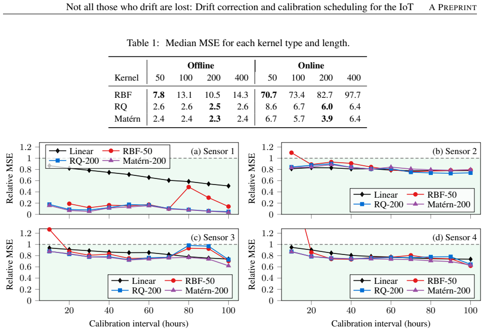
On its own terms, the paper's discovery is that the response function itself, not the sensor output, is the right place to model drift. For dissolved oxygen sensors with affine response $g(y;\beta)=\beta_0+\beta_1 y$, drift appears as slow time variation in the baseline $\beta_0$ and sensitivity $\beta_1$; modeling each coefficient as a Gaussian Process over time, with calibration standard errors as observation noise, yields a corrected analyte estimate $\hat{y}_t=(x_t-\beta_0(t))/\beta_1(t)$ together with a prediction variance. The paper further claims that the same prediction variance can drive calibration scheduling: under a fixed total calibration budget, intervals are shortened for high-uncertainty sensors and lengthened for stable ones, reducing network-wide MSE. With the Matérn kernel, offline correction beat stepwise and linear interpolation on three of four sensors and achieved its largest gains on the most drift-prone sensor. Online, the method matched carrying forward the last calibration for three sensors and improved only the most drifty one by about 30% on average.
Load-bearing premise
The paper assumes each response-function coefficient changes smoothly over time, so a Gaussian Process with a fixed kernel and length scale can interpolate between sparse calibrations; if drift is abrupt or happens far faster than the calibration interval, the correction collapses to carrying the last calibration forward.
Editorial extensions
If this is right
- Historical datasets from drifting sensors can be reanalyzed offline with only a few calibrations, recovering accuracy that would otherwise require a full recalibration campaign.
- Under a fixed calibration budget, network operators can shift calibrations from stable to unstable sensors and expect lower total error without spending more.
- The same per-coefficient Gaussian process machinery transfers to any sensor whose drift can be described as smooth change in a parametrized response function, not just dissolved oxygen sensors.
- Prediction uncertainty from the Gaussian process provides a principled criterion for deciding when a sensor actually needs recalibration, replacing fixed time intervals.
Reading between the lines
- If smoothness is the binding assumption, a natural extension is to compare Gaussian process predictive variance against a threshold and trigger calibrations only when the variance grows, which the paper's uncertainty measure directly enables.
- The online results for stable sensors suggest that the scheduler's main benefit may come in regimes where calibrations are frequent enough for the Gaussian process to track drift; the 15.7% figure includes offline-corrected predictions, so the combined online benefit of scheduler and drift correction remains untested.
- One testable extension is to apply the scheduler's uncertainty allocation to non-affine or multi-analyte response functions, where each coefficient has its own drift timescale.
Editorial analysis
A structured set of objections, weighed in public.
Referee Report
Summary. The paper proposes a Gaussian-process-regression (GPR) drift correction method that models each response-function coefficient as a smooth function of time using calibration measurements and their uncertainties, then inverts the response function to estimate analyte concentration. It also proposes an uncertainty-driven calibration scheduling algorithm (Algorithm 1) that reallocates a fixed calibration budget across sensors according to a GPR-based uncertainty score. The methods are evaluated on four electrochemical dissolved-oxygen sensors over 406 hours against an independent Firesting optical reference, reporting offline MSE reductions of up to 90% and more than 20% on average, plus a further 11.4% network-wide MSE reduction from scheduling (15.7% excluding the 10-hour interval). The online evaluation, however, shows no improvement over stepwise interpolation for three of the four sensors.
Significance. If the offline results are robust, the proposed method would be a valuable, data-efficient drift-correction approach for chemical sensors, requiring only a small number of calibrations and providing calibrated uncertainty estimates. The use of real multi-sensor data with an independent reference, the comparison against stepwise and linear interpolation, and the explicit incorporation of calibration uncertainty are clear strengths. However, the headline numbers are currently supported only by an evaluation in which the GPR hyperparameters are selected on the same data used to report accuracy, so the magnitude of the claimed improvements is not yet established.
major comments (3)
- [Section 5.2.1 and Tables 1-2] The GPR kernel type and length are selected by minimizing median MSE over the same four sensor records and calibration intervals that are subsequently used to report the headline 'up to 90%' and '>20%' MSE reductions in Table 2. The 50 repetitions in Section 5.2 only randomize the first calibration time; every repetition uses the same 406-hour records, so the repetitions do not create independent test sets. This in-sample hyperparameter selection is likely to inflate the reported gains, and the instability of the chosen configuration is visible in Table 2, where RBF-50 gives a relative MSE of 512.73 for Sensor 1 at interval 10. Please provide a genuine held-out evaluation, for example nested cross-validation over calibration intervals or a separate validation period, and report the distribution of relative MSE across independent splits.
- [Section 5.2.3 and Abstract] The abstract claims MSE reductions of up to 90% and more than 20% on average without specifying offline versus online operation, but the online evaluation in Section 5.2.3 and Fig. 9 shows that for sensors 2, 3, and 4 the best kernel yields average relative MSE of 0.98, 1.01, and 0.98, i.e., essentially no improvement over stepwise interpolation. The central claim should be restricted to offline drift correction, or the online method should be improved and evaluated before claiming general applicability.
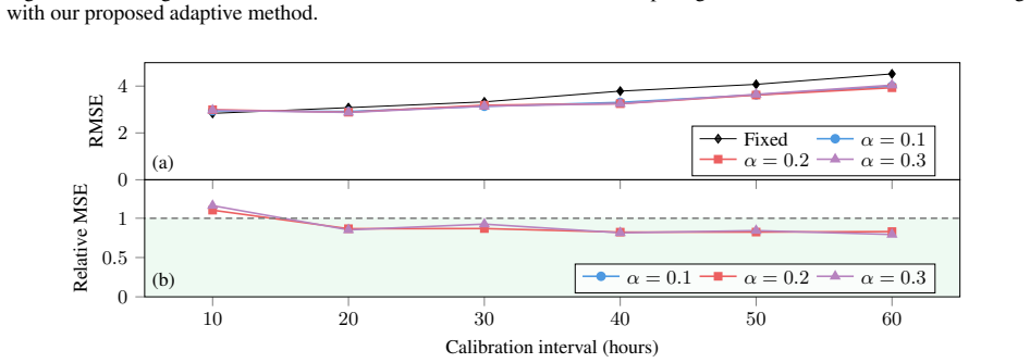
- [Section 5.3 and Table 3] The calibration-scheduling improvement of 11.4% (15.7% excluding the 10-hour interval) is reported after selecting the learning rate alpha and the update frequency on the same data used to quantify the improvement; no held-out period is used. In addition, the uncertainty score u(t_i) in Eq. (17) contains an ad hoc 1/n^2 normalizer whose influence on the scheduling result is never tested. Please evaluate scheduling with a validation protocol that separates configuration selection from reporting, and include a sensitivity analysis for this normalizer.
minor comments (6)
- [Section 2.2, Eq. (7)-(10)] The notation sigma^T_y I in Eqs. (7)-(10) and sigma^T_i I in Eqs. (12)-(13) is not correct for a noise covariance matrix; the noise variances should be placed on the diagonal of a covariance matrix, for example diag(sigma_y) or a separate covariance matrix.
- [Figure 2 caption] The caption lists '(d) corrected data and (e) residuals' but the parenthetical labels repeat '(e)' for the corrected data; the corrected data panel should be labeled (d).
- [Section 5.2.3] There is a typo in the last paragraph: 'calibration invervals' should be 'calibration intervals', and 'as is Section 5.2' should be 'as in Section 5.2'.
- [References] Reference [11] lists the first author as 'C. E. Rasmusen'; the correct spelling is 'Rasmussen'.
- [Section 5.2 and 5.3] The paper reports medians and means across the 50 or 100 repetitions but gives no confidence intervals or error bars. Because the repetitions are not independent (they reuse the same sensor records), error bars would be helpful for assessing whether the reported differences are meaningful.
- [General] No code or data repository is provided. For a methods paper, releasing the dataset and implementation would substantially improve reproducibility and allow independent verification of the reported numbers.
Circularity Check
Headline MSE gains are partly in-sample after hyperparameter selection; the GPR drift-correction derivation itself is not definitionally circular.
-
fitted input called prediction
[Section 5.2.1 (Table 1) and Section 5.2.2 (Table 2/Fig. 8)]
"Table 1 shows the median MSE for each kernel type and length evaluated across all sensors and interval lengths for both offline and online scenarios. As can be seen, a kernel length of 50 hours is most suitable for the RBF kernel, while 200 hours delivers optimal performance when using either RQ and Mat´ern kernels. ... We therefore continue with these parameter values for the remainder of our evaluation. ... Sensor 1 exhibits the greatest MSE reductions due to drift correction using our approach, with the Mat´ern kernel able to reduce MSE by over 90% on average."
The kernel type and length (RBF-50, RQ-200, Matérn-200) are selected by minimizing median MSE in Table 1, which is computed over the same sensors, calibration intervals, and repetitions that are later used in Table 2 and Fig. 8 to report the 'up to 90%' and '>20% average' MSE reductions. Thus the reported headline performance is obtained after choosing the configuration that already scored best on the evaluation set; the performance claim is in-sample after model selection and is statistically forced by the selection criterion rather than being an independent test of the drift-correction method. This is a partial fitted-input-called-prediction issue, although the GPR equations themselves are not definitionally identical to the MSE target.
-
fitted input called prediction
[Section 5.3 (Table 3, Fig. 11)]
"We tested calibration intervals from 10 to 60 in increments of 10 hours and alpha values from 0.05 to 0.4 in increments of 0.05. Each combination was repeated 100 times with random initial calibration times, as is Section 5.2. ... it appears that α = 0.1 performs best with a mean reduction in overall MSE of 11.4%. Excluding 10 hour initial intervals, this increases to 15.7%."
The learning rate α is selected after inspecting RMSE/relative-MSE results for all tested α values on the same evaluation data, and it is also conditional on the kernels and lengths already selected in Section 5.2.1 using the same data. The reported '11.4%' and '15.7%' network-wide improvements are therefore the best values from an in-sample grid search rather than an unbiased, pre-registered estimate of the scheduling method's benefit. This is a fitted-input selection issue: the reported improvement is the maximum over the tuned hyperparameters, not an independent prediction of the method's performance.
full rationale
The core derivation is not circular: GPR models response-function coefficients using calibration data and their uncertainties (Eqs. 11-13), the corrected concentration is obtained by inverting the response function (Eqs. 14-15), and the results are compared with an independent optical reference (Firesting). The calibration scheduler allocates effort according to GPR uncertainty u(ti) (Eq. 17), which is not the same quantity as the reported RMSE/MSE, so the 11.4% improvement is an empirical claim rather than a definitional identity. The only self-citation (Ref. [10], by author Koren) supports background statements about biofouling and is not load-bearing. The 1/n^2 normalizer in Eq. 17 is a heuristic design choice, but because u is not the evaluation metric, it is not definitionally circular. The genuine circularity concern is in the evaluation protocol: kernel type/length (Section 5.2.1) and α (Section 5.3) are selected by minimizing the same MSE/relative-MSE metrics that are then reported as the headline gains, making those quantitative claims in-sample after model selection. This is a fitted-input-called-prediction issue that partially compromises the reported numbers, but it does not make the GPR drift-correction derivation equivalent to its inputs.
Assumptions & free parameters
free parameters (6)
- GPR kernel length scale (ell) =
RBF 50 h; RQ 200 h; Matérn 200 h
- GPR kernel variance and other kernel hyperparameters =
Set by maximizing log marginal likelihood; exact values not reported
- Calibration schedule learning rate alpha =
0.1 chosen as best; grid 0.05 to 0.4 tested
- Uncertainty normalizer 1/n^2 in Eq. 17 =
n is number of calibrations; exponent 2 chosen by hand
- Synchronization offset coefficients in Eq. 18 =
0.129, 24.5, -123.9
- Update frequency for calibration intervals =
once per hour
assumptions (5)
- domain assumption Sensor response is affine over the operating range: g(y; beta) = beta0 + beta1*y.
- domain assumption The response-function coefficients beta0(t) and beta1(t) vary smoothly over time between calibrations.
- domain assumption Calibration standard errors from linear regression accurately represent the noise variances for GPR.
- domain assumption The Firesting optical reference sensor is an accurate ground truth after the correlation-based clock offset correction.
- standard math GPR posterior formulas (Eqs. 8-10) and marginal-likelihood hyperparameter fitting are standard and correctly applied.
invented entities (1)
-
Uncertainty-based calibration priority score u(t_i) (Eq. 17)
Cite this review
Pith. "Pith review of Not all those who drift are lost: Drift correction and calibration scheduling for the IoT." pith.science (2026). https://pith.science/paper/37IPOTPR
@misc{pith2026250609186,
  author       = {Pith},
  title        = {Pith review of: Not all those who drift are lost: Drift correction and calibration scheduling for the IoT},
  year         = {2026},
  howpublished = {\url{https://pith.science/paper/37IPOTPR}},
  note         = {Machine review of arXiv:2506.09186}
}
read the original abstract
Sensors provide a vital source of data that link digital systems with the physical world. However, as sensors age, the relationship between what they measure and what they output changes. This is known as sensor drift and poses a significant challenge that, combined with limited opportunity for re-calibration, can severely limit data quality over time. Previous approaches to drift correction typically require large volumes of ground truth data and do not consider measurement or prediction uncertainty. In this paper, we propose a probabilistic sensor drift correction method that takes a fundamental approach to modelling the sensor response using Gaussian Process Regression. Tested using dissolved oxygen sensors, our method delivers mean squared error (MSE) reductions of up to 90% and more than 20% on average. We also propose a novel uncertainty-driven calibration schedule optimisation approach that builds on top of drift correction and further reduces MSE by up to 15.7%.
Figures


Figures from the paper (8 more)




Reference graph
Works this paper leans on
-
[1]
A review paper on wireless sensor network techniques in internet of things (IoT),
K. Gulati, R. S. Kumar Boddu, D. Kapila, S. L. Bangare, N. Chandnani, and G. Saravanan, “A review paper on wireless sensor network techniques in internet of things (IoT),” Materials Today: Proceedings, vol. 51, pp. 161–165, 2022
work page 2022
-
[2]
Internet of Things architecture challenges: A systematic review,
T. S. Nikoui, A. M. Rahmani, A. Balador, and H. H. S. Javadi, “Internet of Things architecture challenges: A systematic review,”International Journal of Communication Systems, vol. 34, no. 4, 2020
work page 2020
-
[3]
Challenges and opportunities in calibrating low-cost environmental sensors,
N. V . S. R. Nalakurthi, I. Abimbola, T. Ahmed, I. Anton, K. Riaz, Q. Ibrahim, A. Banerjee, A. Tiwari, and S. Gharbia, “Challenges and opportunities in calibrating low-cost environmental sensors,” Sensors, vol. 24, no. 11, p. 3650, 2024
work page 2024
-
[4]
Autonomous in situ calibration of ion-sensitive field effect transistor pH sensors,
P. J. Bresnahan, Y . Takeshita, T. Wirth, T. R. Martz, T. Cyronak, R. Albright, K. Wolfe, J. K. Warren, and K. Mertz, “Autonomous in situ calibration of ion-sensitive field effect transistor pH sensors,” Limnology and Oceanography: Methods, vol. 19, no. 2, pp. 132–144, 2021
work page 2021
-
[5]
To calibrate or not to calibrate, that is the question,
O. Samuelsson, E. U. Lindblom, A. Bj ¨ork, and B. Carlsson, “To calibrate or not to calibrate, that is the question,” Water Research, vol. 229, p. 119338, 2023
work page 2023
-
[6]
Continuous recording of blood oxygen tensions by polarogra- phy,
L. C. Clark, R. Wolf, D. Granger, and Z. Taylor, “Continuous recording of blood oxygen tensions by polarogra- phy,”Journal of Applied Physiology, vol. 6, no. 3, pp. 189–193, 1953
work page 1953
-
[7]
N. P. Revsbech, “Simple sensors that work in diverse natural environments: The micro-Clark sensor and biosen- sor family,”Sensors and Actuators B: Chemical, vol. 329, p. 129168, 2021
work page 2021
-
[8]
Y . Wei, Y . Jiao, D. An, D. Li, W. Li, and Q. Wei, “Review of dissolved oxygen detection technology: From laboratory analysis to online intelligent detection,” Sensors, vol. 19, no. 18, p. 3995, Sep. 2019
work page 2019
Show all 41 references
-
[9]
Minreview: Recent advances in the development of gaseous and dissolved oxygen sensors,
Q. Wang, J.-M. Zhang, and S. Li, “Minreview: Recent advances in the development of gaseous and dissolved oxygen sensors,” Instrumentation Science & Technology, vol. 47, no. 1, pp. 19–50, Aug. 2019. 13 Not all those who drift are lost: Drift correction and calibration schedulin...
2019
-
[10]
Let’s talk about slime; or why biofouling needs more attention in sensor science,
K. Koren and C. M. McGraw, “Let’s talk about slime; or why biofouling needs more attention in sensor science,” ACS Sensors, vol. 8, no. 7, pp. 2432–2439, 2023
2023
-
[11]
C. E. Rasmusen and C. K. I. Williams, Gaussian Processes for Machine Learning. The MIT Press, 2006
2006
-
[12]
An intuitive tutorial to Gaussian Process Regression,
J. Wang, “An intuitive tutorial to Gaussian Process Regression,” Computing in Science & Engineering , vol. 25, no. 4, pp. 4–11, 2023
2023
-
[13]
A tutorial on Gaussian process regression: Modelling, exploring, and exploiting functions,
E. Schulz, M. Speekenbrink, and A. Krause, “A tutorial on Gaussian process regression: Modelling, exploring, and exploiting functions,” Journal of Mathematical Psychology, vol. 85, pp. 1–16, 2018
2018
-
[14]
Introduction to Gaussian processes,
D. J. C. MacKay, “Introduction to Gaussian processes,” NATO ASI series F computer and systems sciences, vol. 168, pp. 133–166, 1998
1998
-
[15]
Advances in drift compensation algorithms for electronic nose technology,
L. Ren, G. Cheng, W. Chen, P. Li, and Z. Wang, “Advances in drift compensation algorithms for electronic nose technology,”Sensor Review, vol. 44, no. 6, pp. 733–745, Aug. 2024
2024
-
[16]
Gaussian process based modeling and experimental design for sensor calibration in drifting environments,
Z. Geng, F. Yang, X. Chen, and N. Wu, “Gaussian process based modeling and experimental design for sensor calibration in drifting environments,” Sensors and Actuators B: Chemical, vol. 216, pp. 321–331, 2015
2015
-
[17]
Low-cost outdoor air quality monitoring and sensor calibration: A survey and critical analysis,
F. Concas, J. Mineraud, E. Lagerspetz, S. Varjonen, X. Liu, K. Puolam¨aki, P. Nurmi, and S. Tarkoma, “Low-cost outdoor air quality monitoring and sensor calibration: A survey and critical analysis,” ACM Transactions on Sensor Networks, vol. 17, no. 2, pp. 1–44, 2021
2021
-
[18]
A multivariate temperature drift modeling and compensation method for large-diameter high-precision fiber optic gyroscopes,
X. Zhao, G. Chen, H. Liu, and L. Wang, “A multivariate temperature drift modeling and compensation method for large-diameter high-precision fiber optic gyroscopes,”IEEE Transactions on Instrumentation and Measurement, vol. 71, pp. 1–12, 2022
2022
-
[19]
Temperature drift compensation of fiber strapdown inertial navigation system based on gsa-svr,
S. Zhao, C. Guo, C. Ke, Y . Zhou, and X. Shu, “Temperature drift compensation of fiber strapdown inertial navigation system based on gsa-svr,”Measurement, vol. 195, p. 111117, May 2022
2022
-
[20]
Evaluation of low-cost air quality sensor calibration models,
K. Aula, E. Lagerspetz, P. Nurmi, and S. Tarkoma, “Evaluation of low-cost air quality sensor calibration models,” ACM Transactions on Sensor Networks, vol. 18, no. 4, pp. 1–32, 2022
2022
-
[21]
Simultaneous temperature drift compensation for eddy current displacement sensors used in magnetically levitated rotor,
C. Wang, S. Zheng, B. Han, and Y . Zhang, “Simultaneous temperature drift compensation for eddy current displacement sensors used in magnetically levitated rotor,”IEEE Transactions on Instrumentation and Measure- ment, vol. 71, pp. 1–9, 2022
2022
-
[22]
Drift compensation of commercial water quality sensors using machine learning to extend the calibration lifetime,
P. Khatri, K. K. Gupta, and R. K. Gupta, “Drift compensation of commercial water quality sensors using machine learning to extend the calibration lifetime,” Journal of Ambient Intelligence and Humanized Computing, vol. 12, no. 2, pp. 3091–3099, 2020
2020
-
[23]
Detection and quantification of temperature sensor drift using probabilistic neural networks,
M. Pereira and B. Glisic, “Detection and quantification of temperature sensor drift using probabilistic neural networks,” Expert Systems with Applications, vol. 213, p. 118884, 2023
2023
-
[24]
Calibration update and drift correction for electronic noses and tongues,
A. Rudnitskaya, “Calibration update and drift correction for electronic noses and tongues,” Frontiers in Chem- istry, vol. 6, 2018
2018
-
[25]
Drift correction for gas sensors using multivariate methods,
T. Artursson, T. Ekl ¨ov, I. Lundstr¨om, P. M˚artensson, M. Sj ¨ostr¨om, and M. Holmberg, “Drift correction for gas sensors using multivariate methods,” Journal of Chemometrics, vol. 14, no. 5–6, pp. 711–723, 2000
2000
-
[26]
Drift compensation of gas sensor array data by orthogonal signal correction,
M. Padilla, A. Perera, I. Montoliu, A. Chaudry, K. Persaud, and S. Marco, “Drift compensation of gas sensor array data by orthogonal signal correction,” Chemometrics and Intelligent Laboratory Systems , vol. 100, no. 1, pp. 28–35, 2010
2010
-
[27]
Drift compensation of gas sensor array data by common principal component analysis,
A. Ziyatdinov, S. Marco, A. Chaudry, K. Persaud, P. Caminal, and A. Perera, “Drift compensation of gas sensor array data by common principal component analysis,” Sensors and Actuators B: Chemical , vol. 146, no. 2, pp. 460–465, 2010
2010
-
[28]
An improved algorithm of drift compensation for olfactory sensors,
S. Lu, J. Guo, S. Liu, B. Yang, M. Liu, L. Yin, and W. Zheng, “An improved algorithm of drift compensation for olfactory sensors,” Applied Sciences, vol. 12, no. 19, p. 9529, 2022
2022
-
[29]
Robust domain correction latent subspace learning for gas sensor drift compensation,
D. Yi, L. Zhang, Z. Wang, L. Wang, S. Duan, and J. Yan, “Robust domain correction latent subspace learning for gas sensor drift compensation,” IEEE Transactions on Systems, Man, and Cybernetics: Systems, vol. 53, no. 12, pp. 7668–7680, 2023
2023
-
[30]
Online sensor drift compensation for e-nose systems using domain adaptation and extreme learning machine,
Z. Ma, G. Luo, K. Qin, N. Wang, and W. Niu, “Online sensor drift compensation for e-nose systems using domain adaptation and extreme learning machine,” Sensors, vol. 18, no. 3, p. 742, 2018
2018
-
[31]
Drift compensation for electronic nose by semi-supervised domain adaption,
Q. Liu, X. Li, M. Ye, S. S. Ge, and X. Du, “Drift compensation for electronic nose by semi-supervised domain adaption,” IEEE Sensors Journal, vol. 14, no. 3, pp. 657–665, 2014. 14 Not all those who drift are lost: Drift correction and calibration scheduling for the IoT A PREPRINT
2014
-
[32]
A novel WWH problem-based semi- supervised online method for sensor drift compensation in e-nose,
Z. Liang, L. Zhang, F. Tian, C. Wang, L. Yang, T. Guo, and L. Xiong, “A novel WWH problem-based semi- supervised online method for sensor drift compensation in e-nose,” Sensors and Actuators B: Chemical , vol. 349, p. 130727, 2021
2021
-
[33]
Chemical gas sensor drift compen- sation using classifier ensembles,
A. Vergara, S. Vembu, T. Ayhan, M. A. Ryan, M. L. Homer, and R. Huerta, “Chemical gas sensor drift compen- sation using classifier ensembles,” Sensors and Actuators B: Chemical, vol. 166–167, pp. 320–329, 2012
2012
-
[34]
Gas sensor drift compensation by ensemble of classifiers using extreme learning machine,
P. Das, A. Manna, and S. Ghoshal, “Gas sensor drift compensation by ensemble of classifiers using extreme learning machine,” in 2020 International Conference on Renewable Energy Integration into Smart Grids: A Multidisciplinary Approach to Technology Modelling and Simulation (...
2020
-
[35]
Calibration of MOX gas sensors in open sampling,
J. G. Monroy, A. Lilienthal, J. L. Blanco, J. Gonzalez-Jimenez, and M. Trincavelli, “Calibration of MOX gas sensors in open sampling,” in IEEE Sensors. IEEE, 2012, pp. 1–4
2012
-
[36]
Anand, P
A. Anand, P. Singh, P. K. Srivastava, and M. Gupta, GIS-based analysis for soil moisture estimation via kriging with external drift. Elsevier, 2021, pp. 391–408
2021
-
[37]
Automatic sensor drift detection and correction using spatial kriging and kalman filtering,
D. Kumar, S. Rajasegarar, and M. Palaniswami, “Automatic sensor drift detection and correction using spatial kriging and kalman filtering,” in IEEE International Conference on Distributed Computing in Sensor Systems . IEEE, 2013, pp. 183–190
2013
-
[38]
Spatiotemporal multisensor calibration via gaussian processes moving target tracking,
J. Persic, L. Petrovic, I. Markovic, and I. Petrovic, “Spatiotemporal multisensor calibration via gaussian processes moving target tracking,” IEEE Transactions on Robotics, vol. 37, no. 5, pp. 1401–1415, 2021
2021
-
[39]
Gaussian process regression model for dynamically calibrating and surveilling a wireless low-cost particulate matter sensor network in delhi,
T. Zheng, M. H. Bergin, R. Sutaria, S. N. Tripathi, R. Caldow, and D. E. Carlson, “Gaussian process regression model for dynamically calibrating and surveilling a wireless low-cost particulate matter sensor network in delhi,” Atmospheric Measurement Techniques, vol. 12, no. 9,...
2019
-
[40]
Sensor calibration and hysteresis compensation with het- eroscedastic gaussian processes,
S. Urban, M. Ludersdorfer, and P. van der Smagt, “Sensor calibration and hysteresis compensation with het- eroscedastic gaussian processes,” IEEE Sensors Journal, vol. 15, no. 11, pp. 6498–6506, Nov. 2015
2015
-
[41]
An enhanced prediction model for the on-line monitoring of the sensors using the Gaussian process regression,
S. Lee and J. Chai, “An enhanced prediction model for the on-line monitoring of the sensors using the Gaussian process regression,” Journal of Mechanical Science and Technology, vol. 33, no. 5, pp. 2249–2257, 2019. 15
2019
Reviewed August 7, 2026 · model on record in the stance chip above.
Discussion (0). Sign in to comment.