Functional Tensor Regression

Anru R. Zhang; Fang Yao; Tongyu Li

REVIEW 3 major objections 3 minor 5 references

Functional Tensor Regression

T0 review · 3 major / 3 minor · reviewed 2026-08-07 · deepseek-v4-flash

Challenge this review Re-run · record.json Download PDF Read on arXiv ↗ Review JSON

Pith's one-line read This paper claims that functional tensor regression—estimating a scalar response from a tensor-valued smooth curve—can be solved by a Riemannian Gauss–Newton algorithm with quadratic convergence and near-minimax error in the tensor…

desk verdict A genuinely new functional tensor regression model with a fast algorithm and plausible rates, but the advertised guarantees rely on an initialization condition the paper never verifies. read the letter →

arxiv 2506.09358 v1 pith:KOV6PEV3 submitted 2025-06-11 stat.ME

Tongyu Li , Fang Yao , Anru R. Zhang This is my paper · ORCID

classification stat.ME MSC 62G0862J0562R3015A69

keywords functionaltensorregressionTuckerdecompositionquadraticconvergenceRiemannianGauss–Newtonsmoothingsplinepenaltyrestrictedisometrypropertyneuroimagingminimaxestimation

verification ladder T0 review T1 audit T2 compute T3 formal

The pith

A machine-rendered reading of the paper's core claim, the machinery that carries it, and where it could break.

The reading

This paper proposes a regression model for a scalar response and a covariate that is a tensor-valued function of time: $y = \int_T \langle X(t), B(t)\\rangle\, dt + \varepsilon$. The coefficient $B$ is recovered through a discrete tensor $\Theta$ with low Tucker rank, with a roughness penalty enforcing smooth evolution along the time mode. The paper's central claim is that the proposed functional Riemannian Gauss–Newton algorithm converges quadratically to a neighborhood of the true coefficient and that the final estimator's squared error scales with the tensor dimension rather than the full parameter count. A minimax lower bound is given to show this tensor-dimension rate cannot be improved in general. A reader should care because time-varying tensor covariates arise in neuroimaging and longitudinal studies, where simply tabular tensor regression ignores smooth temporal structure.

What carries the argument

The load-bearing object is the functional Riemannian Gauss–Newton iteration on the manifold of Tucker-rank-$r$ tensors, where Tucker rank means that the tensor can be written as a small core tensor multiplied by orthonormal factor matrices along each mode. At each step, the tangent space is parameterized by a core increment $C$ and mode-wise corrections $D_d$; the penalized quadratic loss is minimized exactly in those coordinates, then the resulting tangent vector is retracted to the manifold by truncated higher-order singular value decomposition. The second-order convergence argument relies on two quantitative ingredients: a functional analog of the tensor restricted isometry property bounding how the covariate map scales tensor norms, and a spline penalty matrix $A_m$ whose smallest eigenvalue is at least $O(p_0^{-1})$, so the roughness penalty is positive definite and well conditioned.

What would settle it

Run the algorithm on a simulated low-rank functional tensor problem where the true coefficient has a very small smallest nonzero singular value in one mode, start from $H_r(Z^*y)$, and record the per-iteration contraction ratio; a ratio near $1/2$ instead of the squared-error halving predicted by Corollary 1 would show the basin condition is not satisfied by that initialization.

Watch

Extended reading notes

Core claim

The central claim is that, under a functional tensor restricted-isometry condition and a suitable start, the functional Riemannian Gauss–Newton iterates satisfy $\|\Theta_{k+1}-\Theta\|_F \le C_1 \|\Theta_k-\Theta\|_F^2 + C_2\eta$, so the error decreases quadratically until it reaches a ball of radius $O(\eta)$ around the truth. The saturation term has the form $\eta^2 = O_{\\mathrm{pr}}(p_0^{1-2\\kappa}C_m + \rho p_0 C_m + (n\\rho)^{-1}p_0(\sum_d p_d r_d + \prod_d r_d))$, and after tuning $\rho$ the final estimator obeys $\|\\hat\\Theta-\\Theta\|_F^2 = O_{\\mathrm{pr}}((p_0^{-2\\kappa}+n^{-1/2}p_0^{1/2})(\sum_d p_d r_d + \prod_d r_d))$, where $O_{\\mathrm{pr}}$ means the bound holds with probability tending to one. A minimax lower bound of the same order in the tensor dimension shows this part of the rate cannot be improved.

Load-bearing premise

The quadratic convergence and the stated error bound hold only when the initial coefficient tensor already lies in a small neighborhood of the truth, and the paper does not prove that its recommended warm start is inside that neighborhood.

Editorial extensions

If this is right

Each iteration at most doubles the number of correct digits once the iterate is in the basin, so the algorithm reaches the statistical error floor in $O(\log\log(1/\eta))$ steps.
The squared estimation error is proportional to $\sum_d p_d r_d + \prod_d r_d$, the effective number of parameters in a Tucker decomposition, not to the ambient tensor size.
Penalizing the functional mode reduces the nonparametric approximation error $p_0^{-2\kappa}$ and controls the noise term, while the minimax lower bound shows the tensor-dimensional part of the rate is optimal.
The plug-in estimate of $B(t)$ achieves integrated squared error of order $p_0^{-2\kappa} + n^{-1/2}p_0^{1/2}$ relative to the norm of $B$.
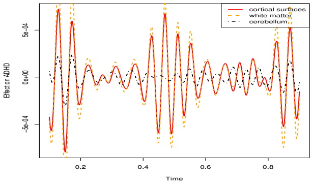
The roughness penalty gives numerical gains over plain tabular tensor regression in simulations and makes the ADHD neuroimaging analysis computationally feasible with only $n=50$ subjects.

Reading between the lines

Editorial extensions of the paper, not claims the author makes directly.

The theory leaves open whether the recommended warm start $H_r(Z^*y)$ actually lies in the basin; one testable extension is to prove a high-probability basin-entry guarantee for a spectral initialization, or to add a safeguarded initial phase.
Because the functional mode enters only through a fixed spline basis and quasi-uniform grid, the same proof structure should extend to irregular grids or to reproducing-kernel penalties, with the constants reworked.
The minimax lower bound is stated for tensor dimensionality only, so a full minimax rate over a Sobolev class of $B(t)$ is still open; the paper's rate suggests such a bound would mix $p_0^{-2\kappa}$ with the tensor-dimension term.
One can check the basin empirically by comparing runs from random starts with runs from $H_r(Z^*y)$: if quadratic convergence is rare from random starts, the local nature of the guarantee is the practical bottleneck.

Share X Bluesky LinkedIn Reddit HN

Signed reviews

No signed human review yet.

Editorial analysis

A structured set of objections, weighed in public.

Desk editor's note, referee report, and a circularity audit.

Desk Editor's Note

read the letter

This paper extends tensor regression to covariates with one smooth functional mode, and it does so in a way that is genuinely new. The model is natural, the roughness penalty is handled inside a Riemannian Gauss–Newton update, and the per-iteration cost is acceptable. The central claims—quadratic convergence and a near-minimax error bound—are structurally plausible because they follow the Luo & Zhang (2023) machinery, which one of the authors knows well. Proposition 1, giving the explicit normal equations for the penalty term, is real work and not a trivial tweak. The theory also separates approximation error, regularization bias, and noise, producing the rate (25) that sensibly trades off smoothing against tensor dimensionality. The simulation study is honest; the functional method beats tabular tensor regression by about 1% in RISE, a small gain that the authors explicitly acknowledge. That is acceptable for a methodological contribution.

The soft spots are real but not fatal. The largest one is initialization. Theorem 1 and Corollary 1 require the initial iterate to lie in a basin whose radius contains λ_min = min_d σ_{r_d}(M_d(Θ)), and for an exact-rank tensor this quantity can be arbitrarily small. The suggested initialization Θ_0 = H_r(Z^* y) is not analyzed, and the stress-test concern is valid: ||H_r(Z^* y)|| generically grows with n while the basin radius, as stated, does not. The paper needs to either prove the basin condition for a reasonable data-generating process or visibly qualify the theorem. Second, the proofs are deferred to a supplementary file that is not included in the arXiv submission, so the theorems cannot currently be verified. That is an editorial problem and should be fixed before publication. Third, the real-data R^2 of 0.991 on n=50 subjects is likely overfit; the cross-validation comparison with ρ=10^-2 helps, but the language describing the fit should be toned down.

This paper deserves a serious referee. The core model and algorithm are new, the rates are plausible, and the initialization gap is a revision issue rather than a desk-reject issue. I would send it to someone with expertise in both tensor optimization and functional data analysis, and would ask the authors to provide the supplementary proofs and to address the initialization condition directly.

Referee Report

3 major / 3 minor

Summary. The paper introduces functional tensor regression, in which a scalar response y is modeled as ∫_T ⟨X(t),B(t)⟩dt + ε with X(t) a functional tensor covariate and B(t) a smooth functional tensor coefficient. The coefficient is discretized on a grid through natural splines, B(t)=Θ×_0{ψ(t)^⊤(Ψ^⊤Ψ)^{-1}Ψ^⊤}, and Θ is assumed to have Tucker rank r. The estimator minimizes the penalized least squares objective (9), L(Θ)+ρJ(Θ), where J enforces smoothness along the functional mode. Estimation is performed by a functional Riemannian Gauss–Newton algorithm (Algorithm 1) that combines the exact tangent-space solve (14) with T-HOSVD retraction (16). The main theoretical results are Theorem 1 (one-step contraction), Corollary 1 (quadratic convergence to a neighborhood of the truth), Theorem 2 (the size of the statistical error η), and Theorem 3 (a minimax lower bound). The paper reports simulation evidence and an ADHD fMRI data analysis. Technical proofs are deferred to an online supplement.

Significance. The proposed estimator and algorithm are potentially significant: if the local convergence theory holds, this is the first functional tensor regression method with a second-order convergence guarantee, and the error bound (25) exhibits a plausible trade-off between the nonparametric smoothing error p0^{-2κ} and the tensor statistical error n^{-1/2}p0^{1/2}(Σ p_d r_d + ∏ r_d). The paper is also usefully accompanied by code and a real-data illustration. My main reservation is not about the overall strategy but about the gap between the theory and the algorithm as actually initialized: the convergence theorems require an initialization basin that the suggested warm start H_r(Z^*y) is not shown to satisfy, and a key lower isometry condition in Lemma 1 is not verified for the iterates. Because these conditions enter the contraction factor and the final bound, the central claim of provable quadratic convergence is not yet fully supported for the recommended implementation.

major comments (3)

[Section 3, Remark 1; Corollary 1; Eq. (25)] The initialization condition is not verified for the recommended Θ0 = H_r(Z^*y). Corollary 1 and hence the final bound (25) require ||Θ0 − Θ||_F to be of order min{ζ_m, D^{-3/2} R_u^{-1/2} R_l^{1/2} λ_min}, where λ_min = min_d σ_{r_d}(M_d(Θ)). The map H_r is homogeneous, while Z^*y = Σ_i y_i Z_i has Frobenius norm of order at least √n (and typically of order n when the signal part of y_i has nonzero mean), with Θ and λ_min fixed; moreover λ_min can be arbitrarily small for a tensor of exact Tucker rank r. Thus H_r(Z^*y) can lie far outside the basin required by Theorem 1, and neither the quadratic convergence phase nor the O_pr(·) bound in (25) is established for the algorithm as used in Section 4. The authors should either prove that this warm start lies in the basin under Assumptions 1–3, or analyze a normalized or projected initialization, or restate the guarantees as conditional on an initialization that is verifiably in the basin.
[Section 3, Lemma 1 and Theorem 1] The lower isometry condition (19) is required at Υ = \checkΘ_{k+1} − Θ, but this difference does not lie in the low-rank manifold M_r: \checkΘ_{k+1} is in the tangent space T_{Θ_k}M_r, so its matricizations can have rank larger than r. Condition (18) is therefore not automatic, and Lemma 2 only gives a sufficient condition involving the singular values of Φ^⊤U_0 and the coefficient α for the leading r_0 columns of M_0(Υ). No argument is supplied that the iterates of Algorithm 1 satisfy (18) with a uniform constant c. Since R_l appears in the contraction factor and in the basin radius, this is a second gap in the induction used to derive Theorem 1 and Corollary 1. The paper should either prove (18) for the relevant Υ under Assumptions 1–3, or state an explicit high-level condition and verify it for the proposed algorithm.
[Section 3, Theorem 3] The minimax lower-bound statement is not in standard form. It asserts a bound on sup_{n≤∏ p_d} n^{1/2} p0^{-1/2} sup_{(y,Z,Θ)∈M} ||\tildeΘ−Θ||_F, with the supremum taken over varying sample sizes n. A minimax lower bound should fix n and give a lower bound on the minimax risk as a function of n (or on the risk multiplied by a known rate). With the supremum over n, the statement could be satisfied by a single favorable n and does not establish that the rate in (25) is unavoidable for every n in the range. Please restate Theorem 3 for fixed n and make explicit how it compares with the upper bound (25).

minor comments (3)

[Algorithm 1 and Remark 1] The pseudocode says 'Initialize Θ0 = S0 × ...' but does not specify how S0 and U_d^0 are obtained, while Remark 1 recommends Θ0 = H_r(Z^*y). Please align the pseudocode with the practical initialization used in Section 4.
[Section 4.1, Figure 2] The caption of the middle panel states 'RISE ∝ n^{-1/2}', but the theoretical relative error in (26) is O_pr(p0^{-2κ} + n^{-1/2} p0^{1/2}); the dashed line may not match the displayed setting unless p0 and κ are specified. Please clarify how the theoretical curve is computed.
[Acknowledgment] The acknowledgment contains a likely typo: 'Newcorner Stone science foundation' should probably read 'New Corner Stone Science Foundation'.

Circularity Check

0 steps flagged · score 0.0 of 10

No significant circularity: the functional tensor regression estimator and its error bounds are derived from stated model assumptions and independent Riemannian Gauss–Newton machinery, not from fitted values or self-referential definitions.

full rationale

The derivation chain is not circular. The target parameter Θ is defined by the spline interpolation (3) and the penalized loss (9), independently of the algorithm; the tuning parameters ρ and r are selected by GCV and are not used as inputs in the theoretical bounds. Theorem 1 and Corollary 1 state conditional convergence guarantees under the RIP-type inequalities (17)–(19), the basin condition ∥Θ0−Θ∥F ≤ ζm, and a nonzero λmin; these conditions are not equivalent to the error bound (25), which follows from Theorem 2's bound on η and Corollary 1's two-phase estimate. The reliance on Luo & Zhang (2023) is substantial but is an external published source for the Riemannian Gauss–Newton projection (11)–(13), the initialization condition, and a norm bound for random low-rank tensors; its assumptions do not include the functional tensor response model or the penalty (6), so it is independent support rather than a self-referential premise. The main genuine weakness is that Remark 1 concedes the recommended initializer Θ0=Hr(Z∗y) is not proven to satisfy the basin condition, so the quadratic convergence phase is conditional on an unverified initialization; this is a completeness/correctness limitation, not a circular step.

Assumptions & free parameters 2 free parameters · 7 assumptions · 0 invented entities

The central theoretical results rest on standard functional data assumptions (Karhunen-Loève expansion, spectral decay, noise structure), an exact low Tucker rank assumption, and the spline interpolation representation of B(·). No invented entities are introduced. The only practical free parameters are the smoothing parameter ρ and the Tucker rank r, both selected by GCV in the numerical studies.

free parameters (2)

smoothing parameter ρ = selected via GCV in Section 4.1; theory uses ρ ≍ (p_0/n)^{1/2}
The estimator and its error rate depend on the choice of ρ; the paper uses GCV in practice and specifies an asymptotic order in the theory. This is a tuning parameter, not a constant fit to data.
Tucker rank r = (r_0, ..., r_D) = selected via GCV in Section 4.1; assumed known in theory
The low-rank constraint is central to the model and all rates. In theory it is fixed and exact; in practice it is selected by minimizing GCV, which is a data-dependent choice.

assumptions (7)

domain assumption Karhunen-Loève expansion (1) of the functional tensor covariate exists with uncorrelated tensor coefficients Ξ_k and orthonormal basis φ_k.
Stated in Section 2.2; standard in functional data analysis but imposes a specific eigenstructure on the covariate process.
domain assumption Assumption 1: E⟨Ξ_k, Υ⟩^2 decays as k^{-a} with a>1, uniformly bounded below and above by A^{-1}k^{-a} and A k^{-a}.
Controls the spectrum of the tensor covariate; needed for Lemma 1's RIP-type bounds.
domain assumption Assumption 2: the discretized eigenfunction matrices Φ_ℓ have bounded spectral norm.
Ensures the functional mode is well-behaved under sampling; needed for Lemma 1 and condition (18).
domain assumption Assumption 3: observation noise E_ij has uncorrelated zero-mean entries with finite variance.
Standard measurement error model for the discretized covariate; used in Lemma 1.
domain assumption The true coefficient parameter Θ lies exactly on the low Tucker rank manifold M_r with known rank r=(r_0,...,r_D).
Assumed in Section 2.3; the estimator and all rates depend on r being correct and low.
ad hoc to paper B(·) is representable as a natural spline interpolant through the grid points (Eq. 3) of order 2m.
This finite-dimensional representation is imposed for simplicity (Section 2.2) and is not a consequence of the Sobolev assumption; approximation error is later absorbed into δ_i.
domain assumption X(·) is almost surely κ-Hölder continuous (0<κ≤1) and ε ~ N(0, σ_y^2) for Theorem 2.
Hölder continuity controls the quadrature approximation error; normality gives the light-tailed bound on (Z^* ε).

how reviews work

0 comments

Cite this review

Pith. "Pith review of Functional Tensor Regression." pith.science (2026). https://pith.science/paper/KOV6PEV3

@misc{pith2026250609358,
  author       = {Pith},
  title        = {Pith review of: Functional Tensor Regression},
  year         = {2026},
  howpublished = {\url{https://pith.science/paper/KOV6PEV3}},
  note         = {Machine review of arXiv:2506.09358}
}

read the original abstract

Tensor regression has attracted significant attention in statistical research. This study tackles the challenge of handling covariates with smooth varying structures. We introduce a novel framework, termed functional tensor regression, which incorporates both the tensor and functional aspects of the covariate. To address the high dimensionality and functional continuity of the regression coefficient, we employ a low Tucker rank decomposition along with smooth regularization for the functional mode. We develop a functional Riemannian Gauss--Newton algorithm that demonstrates a provable quadratic convergence rate, while the estimation error bound is based on the tensor covariate dimension. Simulations and a neuroimaging analysis illustrate the finite sample performance of the proposed method.

Figures

Figures reproduced from arXiv: 2506.09358 by the authors.

**Figure 2.** Left: RISE versus the standard deviation of errors. Displayed are averages based [PITH_FULL_IMAGE:figures/full_fig_p026_2.png] view at source ↗

**Figure 3.** Functional tensor regression applied to the ADHD data. Plotted are slices from [PITH_FULL_IMAGE:figures/full_fig_p028_3.png] view at source ↗

Figures from the paper (1 more)

**Figure 4.** Figure 4: Estimated effects of different regions of the brain on ADHD along time. [PITH_FULL_IMAGE:figures/full_fig_p029_4.png]

Discussion (0). Continue with ORCID to comment.

Reference graph

Works this paper leans on

5 extracted references · 5 canonical work pages

[1]

& Sepulchre, R

Absil, P.-A., Mahony, R. & Sepulchre, R. (2009),Optimization algorithms on matrix man- ifolds, Princeton University Press. Ahmed, T., Raja, H. & Bajwa, W. U. (2020), ‘Tensor regression using low-rank and sparse tucker decompositions’,SIAM Journal on Mathematics of Data Science2(4), 944–966. Bi, X., Qu, A. & Shen, X. (2018), ‘Multilayer tensor factorizatio...

work page 2009
[39]

Bayesian tensor regression using the Tucker decomposition for sparse spatial modeling

Luo, Y., Tao, D., Ramamohanarao, K., Xu, C. & Wen, Y. (2015), ‘Tensor canonical cor- relation analysis for multi-view dimension reduction’,IEEE transactions on Knowledge and Data Engineering27(11), 3111–3124. Luo, Y. & Zhang, A. R. (2023), ‘Low-rank tensor estimation via riemannian gauss-newton: Statistical optimality and second-order convergence’,Journal...

work page Pith review arXiv 2015
[1169]

& Xia, D

Jing, B.-Y., Li, T., Lyu, Z. & Xia, D. (2021), ‘Community detection on mixture multilayer networks via regularized tensor decomposition’,The Annals of Statistics49(6), 3181–

work page 2021
[1402]

Eubank, R. L. (1999),Nonparametric regression and spline smoothing, CRC press. Gandy, S., Recht, B. & Yamada, I. (2011), ‘Tensor completion and low-n-rank tensor recovery via convex optimization’,Inverse problems27(2), 025010. Goldfarb, D. & Qin, Z. (2014), ‘Robust low-rank tensor recovery: Models and algorithms’, SIAM Journal on Matrix Analysis and Appli...

work page 1999
[3205]

& Cipolla, R

Kim, T.-K., Wong, S.-F. & Cipolla, R. (2007), Tensor canonical correlation analysis for action classification,in‘2007 IEEE Conference on Computer Vision and Pattern Recog- nition’, IEEE, pp. 1–8. Koch, O. & Lubich, C. (2010), ‘Dynamical tensor approximation’,SIAM Journal on Matrix Analysis and Applications31(5), 2360–2375. Kolda, T. G. & Bader, B. W. (200...

work page 2007

Pith tools

Reviewed August 7, 2026 · model on record in the stance chip above.

[1] [1]

& Sepulchre, R

Absil, P.-A., Mahony, R. & Sepulchre, R. (2009),Optimization algorithms on matrix man- ifolds, Princeton University Press. Ahmed, T., Raja, H. & Bajwa, W. U. (2020), ‘Tensor regression using low-rank and sparse tucker decompositions’,SIAM Journal on Mathematics of Data Science2(4), 944–966. Bi, X., Qu, A. & Shen, X. (2018), ‘Multilayer tensor factorizatio...

work page 2009

[2] [39]

Bayesian tensor regression using the Tucker decomposition for sparse spatial modeling

Luo, Y., Tao, D., Ramamohanarao, K., Xu, C. & Wen, Y. (2015), ‘Tensor canonical cor- relation analysis for multi-view dimension reduction’,IEEE transactions on Knowledge and Data Engineering27(11), 3111–3124. Luo, Y. & Zhang, A. R. (2023), ‘Low-rank tensor estimation via riemannian gauss-newton: Statistical optimality and second-order convergence’,Journal...

work page Pith review arXiv 2015

[3] [1169]

& Xia, D

Jing, B.-Y., Li, T., Lyu, Z. & Xia, D. (2021), ‘Community detection on mixture multilayer networks via regularized tensor decomposition’,The Annals of Statistics49(6), 3181–

work page 2021

[4] [1402]

Eubank, R. L. (1999),Nonparametric regression and spline smoothing, CRC press. Gandy, S., Recht, B. & Yamada, I. (2011), ‘Tensor completion and low-n-rank tensor recovery via convex optimization’,Inverse problems27(2), 025010. Goldfarb, D. & Qin, Z. (2014), ‘Robust low-rank tensor recovery: Models and algorithms’, SIAM Journal on Matrix Analysis and Appli...

work page 1999

[5] [3205]

& Cipolla, R

Kim, T.-K., Wong, S.-F. & Cipolla, R. (2007), Tensor canonical correlation analysis for action classification,in‘2007 IEEE Conference on Computer Vision and Pattern Recog- nition’, IEEE, pp. 1–8. Koch, O. & Lubich, C. (2010), ‘Dynamical tensor approximation’,SIAM Journal on Matrix Analysis and Applications31(5), 2360–2375. Kolda, T. G. & Bader, B. W. (200...

work page 2007