REVIEW 4 major objections 5 minor 58 references
Time-Varying Home Field Advantage in Football: Learning from a Non-Stationary Causal Process
T0 review · 4 major / 5 minor · reviewed 2026-08-07 · deepseek-v4-flash
Pith's one-line read DYNAMO, a local M-estimator for non-stationary causal discovery, recovers time-varying causal graphs from a single trajectory and attributes Premier League home-field advantage to crowd-dependent referee bias.
desk verdict DYNAMO is a genuine methodological advance for time-varying causal structure learning, but the sports application's referee-bias claims are not identified by the stated assumptions. read the letter →
The pith
A machine-rendered reading of the paper's core claim, the machinery that carries it, and where it could break.
The reading
What carries the argument
The machinery is the locally stationary causal process model paired with a kernel-weighted local M-estimator. For each rescaled time $\tau = t/T$, a kernel $K_h$ with bandwidth $h$ weighs observations within $\tau \pm h$, and the causal parameters $\theta(\tau)$ minimize $L_t(\vartheta) = (Th)^{-1} \sum_l \ell(x_l, Y_{l-1}; \vartheta) K((\tau_l - \tau)/h)$. The key identity is a stationary approximation: under the paper's Lipschitz conditions there exists, for each $\tau$, a stationary process $\tilde{x}_t(\tau)$ with the same causal structure $\theta(\tau)$, and the observed process differs from it by $O(T^{-1} + |\tau_l - \tau|)$. That approximation makes the non-stationary loss converge to the stationary loss, which transfers identifiability results from stationary causal models and yields the consistency rate.
What would settle it
A concrete check is to re-estimate the same graphs with opponent-strength ratings, travel distance, and referee identity added to the conditioning set; if the direct edges from opponent yellow cards and fouls to expected goals disappear or flip sign, Assumption 1 fails and the referee-bias claim does not survive. A second check is a placebo test that randomly relabels home and away in the aggregated series; if DYNAMO still finds home-advantage edges at the same rate, the recovery is not picking up a real match process.
Extended reading notes
Core claim
The central claim is that a single realization of a locally stationary causal process $x_t = f(\mathrm{Pa}(x_t), \epsilon_t; \theta(t/T))$ contains enough local information to identify and consistently estimate the entire evolving causal structure $G_t$, provided the map from time to parameters is smooth in a Lipschitz sense. DYNAMO minimizes a kernel-weighted M-estimation loss, using the NOTEARS continuous acyclicity constraint for linear graphs and the NTS-NOTEAR neural-network loss for nonlinear graphs; the theory states that as $T h \to \infty$ with $T h^7 \to 0$, the estimated parameters converge to the true ones. On the data side, the application claims that the causal edges from opponent yellow cards and opponent fouls to expected goals, interpreted as referee bias, are time-varying and team-specific, and that their patterns differ sharply between the closed-door 2020-2021 season and the spectator season 2021-2022. This is the paper's evidence that home-field advantage is not a single league-wide constant but a moving set of causal relationships.
Load-bearing premise
The load-bearing premise is that, after taking home-minus-away differences averaged over each team's 38 matches, the measured in-match statistics have no unobserved confounders and behave like a single realization of a locally stationary causal process; if omitted factors such as opponent strength, fatigue, or referee assignment drive both the statistics and expected goals, the referee-bias edges are not causal.
Editorial extensions
If this is right
- Team-level home advantage can be decomposed into minute-by-minute causal pathways, so a club could target specific match phases or opponent habits rather than treating home advantage as one number.
- Referee bias is not constant across match phases; official training and evaluation could focus on the phases where crowd pressure shifts decisions.
- The same estimator applies to any non-stationary observational time series where a single long trajectory is available, not just football.
- Because DYNAMO's learned graphs improve goal prediction over static baselines, the paper implies that causally informed features carry predictive value beyond raw expected-goal aggregates.
- The empty-stadium versus full-stadium seasons provide a natural benchmark: the crowd's effect on home advantage can be read off the changing referee-bias edges.
Reading between the lines
- The natural next test is to run DYNAMO on matches with partial stadium capacity or neutral venues; if referee-bias edges track crowd density continuously, the crowd's causal role is confirmed, whereas if only home/away status matters, the mechanism is not crowd volume.
- The paper aggregates each team's 38 matches into one home-minus-away series, so the team-specific graphs are season averages; applying the method to a single match would be a much harder test and would clarify whether the graphs capture within-match process or between-match selection.
- If the claim transfers beyond sports, the same local-M machinery could estimate time-varying causal structures in economics or epidemiology where stationarity fails, but the unconfoundedness assumption will usually be harder to defend outside event data with rich controls.
- The referee-bias result suggests a record-level falsification: compare estimated officiating edges with actual referee reports or disciplinary actions; if decisions recorded as errors do not correlate with the estimated bias edges, the causal label is in question.
Editorial analysis
A structured set of objections, weighed in public.
Referee Report
Summary. The paper proposes DYNAMO, a kernel-weighted local M-estimator that extends NOTEARS-style structure learning to locally stationary causal processes, with identifiability and consistency theorems, simulation comparisons against several benchmarks, and an application to two English Premier League seasons. The application constructs minute-level home-minus-away difference series per team, estimates time-varying graphs for within-match variables, and interprets edges from opponent fouls and yellow cards to expected goals as evidence of referee bias. It also claims that the learned causal structures improve goal prediction accuracy compared with existing methods.
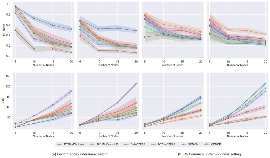
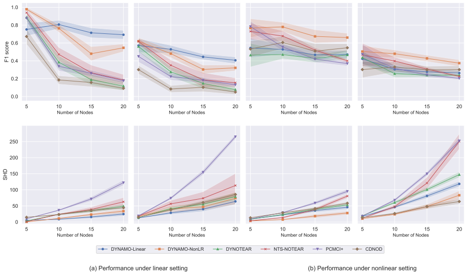
Significance. If the theoretical results hold, the methodological core is a useful contribution: DYNAMO localizes a flexible class of DAG learners and supplies consistency guarantees in the locally stationary setting, and the simulation study is unusually broad, covering linear and nonlinear models, varying node counts and time lengths, faster changes, more lags, and non-Gaussian noise. The comparisons against DYNOTEARS, NTS-NOTEARS, PCMCI+, and CD-NOD are meaningful. The real-data claims, however, are substantially stronger than the evidence: the causal referee-bias interpretation rests on unconfoundedness and on treating cross-match averaged series as a causal process, and the prediction improvement is demonstrated only through an in-sample reconstruction. These gaps affect the paper's central applied claims rather than its local methodological machinery.
major comments (4)
- [Section 3.1 and Appendix D] The causal interpretation of the EPL application is not identified. Assumption 1 rules out unobserved confounders, but the input series defined in Appendix D as X_i^t = (2/N_i) sum_j X^{ij}_t (I(loc_j=1) - I(loc_j=0)) averages 38 matches per minute, so a 'shock' to this series at minute t is cross-match sampling variation rather than a structural intervention within a single match. OF and OY are endogenous match-state variables: a team falling behind commits more fouls and also concedes higher XG, while opponent strength, red cards, tactical setup, and fatigue are common drivers of both OF/OY and XG. Sections 5.1 and 5.3 label direct OF->XG and OY->XG edges as 'referee bias' (Figure 4), but such edges can arise from confounding even when referees are perfectly unbiased. The robustness checks in Appendix D.1 and the in-sample MSE in Table 1 do not control for these drivers; the supplement's own 'Limitation' section calls for more granular referee-bias data such as free kicks and penalties, underscoring that OF and OY are not direct measures of referee decisions.
- [Section 5.2, Table 1] The claim of improved goal prediction accuracy is not supported by Table 1. DYNAMO minimizes squared error against XG using contemporaneous match variables, and the table then compares its fitted values with actual goals, while the baseline XG does not see those contemporaneous variables. This is an in-sample reconstruction comparison, not a predictive evaluation. No holdout matches or time-based split are used, and no confidence intervals accompany the reported MSE values. An out-of-sample evaluation, or a comparison using only information available at prediction time, is required before the abstract's prediction-improvement claim can stand.
- [Section 3.5, Theorem 1, and Supplement C.4.2] The abstract's claim of identifiability 'without imposing additional assumptions' is overstated. Theorem 1 is derived from Lemma C.5, which for additive-noise and post-nonlinear stationary models invokes Assumptions C.6 (causal minimality) and C.7 (well-defined density), and for Gaussian DAGs relies on the equal-error-variance condition of Peters and Buehlmann (2014). These conditions should be stated as assumptions of Theorem 1 in the main text rather than deferred to the supplement, since they are load-bearing for the identifiability result.
- [Section 5.2 and Appendix D.2] The application-level conclusions in Figure 4 are asserted without uncertainty quantification. Each team-season series has T = 90 time points and roughly d = 16 variables, and local estimation uses bandwidths around 0.5-0.9, so each local fit sees only a small fraction of the 90 observations; the asymptotic regime of Theorem 2 (T h -> infinity, T h^7 -> 0) is not directly informative at this sample size. Edges are thresholded at 0.05, but no confidence intervals, bootstrap stability, or false-discovery measures are reported. The second- and third-best bandwidth comparisons in Appendix D.1 show visual agreement but do not quantify the uncertainty of the reported time-varying structures.
minor comments (5)
- [Section 3.1] Assumption 1 is titled 'Unconfoundness'; the standard spelling is 'Unconfoundedness'.
- [Section 3.5 and Theorem 2] Theorem 2 refers to 'the loss in Eq. (1)' but the objective is Eq. (3); the same equation reference is used incorrectly in the consistency statement.
- [Table 1 and Appendix D.1] The header 'DYNOTEAR' is inconsistent with 'DYNOTEARS' elsewhere, and Appendix D.1 contains the typo 'DYNOTEAERS'.
- [Figure 4 and Supplement Figures] The captions say 'Orange notes represent contemporary variables'; 'notes' should be 'nodes'.
- [Algorithm 3] Bandwidth selection randomly divides the time series into folds; for dependent locally stationary data this can place adjacent observations in different folds and overstate effective sample size, so a blocked or leave-one-out scheme consistent with Richter and Dahlhaus (2019) would be safer.
Circularity Check
The goal-prediction validation in Table 1 is an in-sample fit of the very XG series DYNAMO is trained on, so the headline accuracy claim reduces by construction; the referee-bias conclusions rest on an unverified unconfoundedness assumption rather than on circular reasoning.
-
fitted input called prediction
[Section 5.2 (Model Validation), Table 1; Eq. (4)]
"Third, we use our DYNAMO model to predict the expected goals (XG) at each minute and compare these predictions to the actual goals scored. ... L^{lr}_t(W_t,A_t)=\frac{1}{Th}\sum_l \|x_l-W_t^\top x_l-A_t^\top Y_{l-1}\|_2^2 K_h(\tau_l-\tau_t)+\lambda_1\|W_t\|+\lambda_2\|A_t\|+\frac{\alpha}{2}H(W_t)^2+\rho H(W_t)."
The 'predictions' in Table 1 are the fitted values of the XG coordinate of x_l under the same loss (4) that DYNAMO minimizes: the objective includes \|x_l - W_t^\top x_l - A_t^\top Y_{l-1}\|_2^2, so the XG component is the training target, and contemporaneous variables (TS, OF, OY, etc.) are available as regressors. The quasi-k-fold CV in Eq. (6) is used only to choose the bandwidth h, not to produce held-out goal predictions; the table compares these in-sample reconstructions of a 38-match home-minus-away averaged XG series against 'actual goals scored' and against the fixed 'original XG' baseline, which does not use the same contemporaneous covariates. The gap therefore measures fitting flexibility, not predictive or causal validity.
full rationale
The derivation of the DYNAMO estimator itself is largely self-contained: identifiability is reduced to external identifiability results for stationary Gaussian/non-Gaussian, additive-noise, and post-nonlinear models, and the consistency proof invokes generic locally stationary process bounds plus base-learner rates. The simulation studies generate data from the same structural equation model in Eq. (1) with known ground truth, so they are not circular. The genuine circular step is the model-validation claim in Section 5.2 and Table 1: Eq. (4) minimizes squared error of the full vector x_l, including the XG coordinate, using contemporaneous variables as regressors; the 'predictions' compared with 'actual goals scored' are in-sample fitted values from the same 38-match smoothed series, with no held-out split for the comparison. Thus the abstract's 'improve goal prediction accuracy' claim reduces to a fit of the series being predicted. Separately, the referee-bias interpretation of OF-to-XG and OY-to-XG edges is not circular but is an identification risk: it requires Assumption 1 (no unobserved confounders) on an aggregate home-minus-away series and treats endogenous foul and card counts as pure referee inputs. The supplement's own limitation section concedes that more granular referee-bias data such as free kicks and penalty kicks would offer additional insights, underscoring that OF and OY are coarse proxies. These are correctness concerns rather than circularity, so they do not by themselves raise the score beyond 6. The self-citations (Price et al. 2022 for preprocessing; Cai et al. 2023 for a Gaussian-DAG rate) are not load-bearing after the design argument for differencing and the availability of external identifiability theorems.
Assumptions & free parameters
free parameters (4)
- Kernel bandwidth h =
Per team and time point, roughly 0.4 to 0.9
- Sparsity penalties lambda1, lambda2 =
0.05 for linear DYNAMO; 0.005/0.01 for nonlinear DYNAMO
- Edge threshold =
0.05
- Lagged period L =
1 (with a robustness check for L=2)
assumptions (6)
- domain assumption Assumption 1: No unobserved confounders
- domain assumption Assumption 2: The graph G_t is acyclic at each time t
- ad hoc to paper Assumption 3: Locally Stationary Causality (Lipschitz and contraction conditions)
- ad hoc to paper Assumption C.6: Causal Minimality
- domain assumption Assumption C.7: Well-defined density and smoothness
- domain assumption Home-away differencing yields a valid locally stationary causal process of length 90
Cite this review
Pith. "Pith review of Time-Varying Home Field Advantage in Football: Learning from a Non-Stationary Causal Process." pith.science (2026). https://pith.science/paper/IVCBGDYO
@misc{pith2026250611399,
  author       = {Pith},
  title        = {Pith review of: Time-Varying Home Field Advantage in Football: Learning from a Non-Stationary Causal Process},
  year         = {2026},
  howpublished = {\url{https://pith.science/paper/IVCBGDYO}},
  note         = {Machine review of arXiv:2506.11399}
}
read the original abstract
In sports analytics, home field advantage is a robust phenomenon where the home team wins more games than the away team. However, discovering the causal factors behind home field advantage presents unique challenges due to the non-stationary, time-varying environment of sports matches. In response, we propose a novel causal discovery method, DYnamic Non-stAtionary local M-estimatOrs (DYNAMO), to learn the time-varying causal structures of home field advantage. DYNAMO offers flexibility by integrating various loss functions, making it practical for learning linear and non-linear causal structures from a general class of non-stationary causal processes. By leveraging local information, we provide theoretical guarantees for the identifiability and estimation consistency of non-stationary causal structures without imposing additional assumptions. Simulation studies validate the efficacy of DYNAMO in recovering time-varying causal structures. We apply our method to high-resolution event data from the 2020-2021 and 2021-2022 English Premier League seasons, during which the former season had no audience presence. Our results reveal intriguing, time-varying, team-specific field advantages influenced by referee bias, which differ significantly with and without crowd support. Furthermore, the time-varying causal structures learned by our method improve goal prediction accuracy compared to existing methods.
Figures


Figures from the paper (17 more)




Reference graph
Works this paper leans on
-
[1]
Cai, H., Y. Wang, M. Jordan, and R. Song (2023). On learning necessary and sufficient causal graphs. arXiv preprint arXiv:2301.12389\/
work page Pith review arXiv 2023
-
[2]
Dahlhaus, R. and S. S. Rao (2006). Statistical inference for time-varying ARCH processes . The Annals of Statistics\/ 34\/ (3), 1075 -- 1114
work page 2006
-
[3]
Dahlhaus, R., S. Richter, and W. B. Wu (2019). Towards a general theory for nonlinear locally stationary processes . Bernoulli\/ 25\/ (2), 1013 -- 1044
work page 2019
-
[4]
Gao, J., B. Peng, W. B. Wu, and Y. Yan (2024). Time-varying multivariate causal processes. Journal of Econometrics\/ 240\/ (1), 105671
work page 2024
-
[5]
Gao, T., D. Bhattacharjya, E. Nelson, M. Liu, and Y. Yu (2022). Idyno: Learning nonparametric dags from interventional dynamic data. In International Conference on Machine Learning , pp.\ 6988--7001. Pmlr
work page 2022
-
[6]
Rhino: Deep Causal Temporal Relationship Learning With History-dependent Noise
Gong, W., J. Jennings, C. Zhang, and N. Pawlowski (2022). Rhino: Deep causal temporal relationship learning with history-dependent noise. arXiv preprint arXiv:2210.14706\/
work page Pith review arXiv 2022
-
[7]
Hoyer, P., D. Janzing, J. M. Mooij, J. Peters, and B. Sch \"o lkopf (2008). Nonlinear causal discovery with additive noise models. Advances in neural information processing systems\/ 21
work page 2008
-
[8]
Lanne, M., M. Meitz, and P. Saikkonen (2017). Identification and estimation of non-gaussian structural vector autoregressions. Journal of Econometrics\/ 196\/ (2), 288--304
work page 2017
Show all 58 references
-
[9]
Sriwattanaworachai, S
Pamfil, R., N. Sriwattanaworachai, S. Desai, P. Pilgerstorfer, K. Georgatzis, P. Beaumont, and B. Aragam (2020). Dynotears: Structure learning from time-series data. In International Conference on Artificial Intelligence and Statistics , pp.\ 1595--1605. PMLR
2020
-
[10]
Peters, J. and P. B \"u hlmann (2014). Identifiability of gaussian structural equation models with equal error variances. Biometrika\/ 101\/ (1), 219--228
2014
-
[11]
Peters, J., J. M. Mooij, D. Janzing, and B. Sch \"o lkopf (2014). Causal discovery with continuous additive noise models. The Journal of Machine Learning Research\/ 15\/ (1), 2009--2053
2014
-
[12]
Price, K., H. Cai, W. Shen, and G. Hu (2022). How much does home field advantage matter in soccer games? a causal inference approach for english premier league analysis. arXiv preprint arXiv:2205.07193\/
2022 arXiv
-
[13]
Inazumi, Y
Shimizu, S., T. Inazumi, Y. Sogawa, A. Hyvarinen, Y. Kawahara, T. Washio, P. O. Hoyer, K. Bollen, and P. Hoyer (2011). Directlingam: A direct method for learning a linear non-gaussian structural equation model. Journal of Machine Learning Research-JMLR\/ 12\/ (Apr), 1225--1248
2011
-
[14]
Schulte, G
Sun, X., O. Schulte, G. Liu, and P. Poupart (2023). Nts-notears: Learning nonparametric dbns with prior knowledge. In International Conference on Artificial Intelligence and Statistics , pp.\ 1942--1964. PMLR
2023
-
[15]
Zhang, K. and A. Hyv \"a rinen (2009). On the identifiability of the post-nonlinear causal model. In Proceedings of the Twenty-Fifth Conference on Uncertainty in Artificial Intelligence , pp.\ 647--655
2009
-
[16]
Aragam, P
Zheng, X., B. Aragam, P. K. Ravikumar, and E. P. Xing (2018). Dags with no tears: Continuous optimization for structure learning. Advances in neural information processing systems\/ 31
2018
-
[17]
Zheng, X., C. Dan, B. Aragam, P. Ravikumar, and E. Xing (2020). Learning sparse nonparametric dags. In International Conference on Artificial Intelligence and Statistics , pp.\ 3414--3425. PMLR
2020
-
[18]
Albert, J., M. E. Glickman, T. B. Swartz, and R. H. Koning (2017). Handbook of Statistical Methods and Analyses in Sports . Boca Raton, FL: Chapman & Hall/CRC
2017
-
[19]
Aragam, and P
Bello, K., B. Aragam, and P. Ravikumar (2022). Dagma: Learning dags via m-matrices and a log-determinant acyclicity characterization. Advances in Neural Information Processing Systems\/ 35 , 8226--8239
2022
-
[20]
Dolton, J
Bryson, A., P. Dolton, J. J. Reade, D. Schreyer, and C. Singleton (2021). Causal effects of an absent crowd on performances and refereeing decisions during covid-19. Economics Letters\/ 198 , 109664
2021
-
[21]
Forrest, and R
Buraimo, B., D. Forrest, and R. Simmons (2010). The 12th man?: refereeing bias in english and german soccer. Journal of the Royal Statistical Society Series A: Statistics in Society\/ 173\/ (2), 431--449
2010
-
[22]
D’Amour, L
Cervone, D., A. D’Amour, L. Bornn, and K. Goldsberry (2016). A multiresolution stochastic process model for predicting basketball possession outcomes. Journal of the American Statistical Association (Applications and Case Studies)\/ 111\/ (514), 585--599
2016
-
[23]
Courneya, K. S. and A. V. Carron (1992). The home advantage in sport competitions: A literature review. Journal of Sport & Exercise Psychology\/ 14\/ (1), 13--27
1992
-
[24]
Dahlhaus, R. (1996). On the kullback-leibler information divergence of locally stationary processes. Stochastic processes and their applications\/ 62\/ (1), 139--168
1996
-
[25]
Dai, R., J. Wang, F. Zhou, S. Luo, Z. Qin, C. Shi, and H. Zhu (2024). Causal deepsets for off-policy evaluation under spatial or spatio-temporal interferences. arXiv preprint arXiv:2407.17910\/
2024 arXiv
-
[26]
ghost matches
Endrich, M. and T. Gesche (2020). Home-bias in referee decisions: Evidence from “ghost matches” during the covid19-pandemic. Economics Letters\/ 197 , 109621
2020
-
[27]
Koyama, K
Fujiwara, D., K. Koyama, K. Kiritoshi, T. Okawachi, T. Izumitani, and S. Shimizu (2023). Causal discovery for non-stationary non-linear time series data using just-in-time modeling. In Conference on Causal Learning and Reasoning , pp.\ 880--894. PMLR
2023
-
[28]
Addanki, T
Gao, S., R. Addanki, T. Yu, R. A. Rossi, and M. Kocaoglu (2023). Causal discovery in semi-stationary time series. In Thirty-seventh Conference on Neural Information Processing Systems
2023
-
[29]
Goumas, C. (2017). Modelling home advantage for individual teams in uefa champions league football. Journal of sport and health science\/ 6\/ (3), 321--326
2017
-
[30]
Grieshop, N., Y. Feng, G. Hu, and M. Schweinberger (2023). A continuous-time stochastic process for high-resolution network data in sports. arXiv preprint arXiv:2303.01318\/
2023 arXiv
-
[31]
Canniford, and G
Hill, T., R. Canniford, and G. Eckhardt (2023). What makes anfield atmospheric?: Dense interaction ritual chains. In Consuming Atmospheres , pp.\ 91--106. Routledge
2023
-
[32]
Canniford, and G
Hill, T., R. Canniford, and G. M. Eckhardt (2022). The roar of the crowd: How interaction ritual chains create social atmospheres. Journal of Marketing\/ 86\/ (3), 121--139
2022
-
[33]
Hu, G., H.-C. Yang, Y. Xue, and D. K. Dey (2023). Zero-inflated P oisson model with clustered regression coefficients: Application to heterogeneity learning of field goal attempts of professional basketball players. Canadian Journal of Statistics\/ 51 , 157--172
2023
-
[34]
Zhang, M
Huang, B., K. Zhang, M. Gong, and C. Glymour (2019). Causal discovery and forecasting in nonstationary environments with state-space models. In International conference on machine learning , pp.\ 2901--2910. PMLR
2019
-
[35]
Zhang, J
Huang, B., K. Zhang, J. Zhang, J. Ramsey, R. Sanchez-Romero, C. Glymour, and B. Sch \"o lkopf (2020). Causal discovery from heterogeneous/nonstationary data. The Journal of Machine Learning Research\/ 21\/ (1), 3482--3534
2020
-
[36]
Johnston, R. (2008). On referee bias, crowd size, and home advantage in the english soccer premiership. Journal of Sports Sciences\/ 26\/ (6), 563--568
2008
-
[37]
Richter, and W
Karmakar, S., S. Richter, and W. B. Wu (2022). Simultaneous inference for time-varying models. Journal of Econometrics\/ 227\/ (2), 408--428
2022
-
[38]
Moliner-Urdiales, and D
Legaz-Arrese, A., D. Moliner-Urdiales, and D. Mungu \' a-Izquierdo (2013). Home advantage and sports performance: evidence, causes and psychological implications. Universitas Psychologica\/ 12\/ (3), 933--943
2013
-
[39]
Liu, G., Y. Luo, O. Schulte, and P. Poupart (2022). Uncertainty-aware reinforcement learning for risk-sensitive player evaluation in sports game. Advances in Neural Information Processing Systems\/ 35 , 20218--20231
2022
-
[40]
Marek, P. and F. V \'a vra (2020). Comparison of home advantage in european football leagues. Risks\/ 8\/ (3), 87
2020
-
[41]
Nevill, A. M. and R. L. Holder (1999). Home advantage in sport: An overview of studies on the advantage of playing at home. Sports Medicine\/ 28 , 221--236
1999
-
[42]
Pollard, R. (2006). Worldwide regional variations in home advantage in association football. Journal of sports sciences\/ 24\/ (3), 231--240
2006
-
[43]
Rahmani, A. and P. Frossard (2023). Castor: Causal temporal regime structure learning. arXiv preprint arXiv:2311.01412\/
2023 arXiv
-
[44]
Drust, and N
Reilly, T., B. Drust, and N. Clarke (2008). Muscle fatigue during football match-play. Sports Medicine\/ 38 , 357--367
2008
-
[45]
Richter, S. and R. Dahlhaus (2019). Cross validation for locally stationary processes . The Annals of Statistics\/ 47\/ (4), 2145 -- 2173
2019
-
[46]
Cevher, M
Rolland, P., V. Cevher, M. Kleindessner, C. Russell, D. Janzing, B. Sch \"o lkopf, and F. Locatello (2022). Score matching enables causal discovery of nonlinear additive noise models. In International Conference on Machine Learning , pp.\ 18741--18753. PMLR
2022
-
[47]
Runge, J. (2020). Discovering contemporaneous and lagged causal relations in autocorrelated nonlinear time series datasets. In Conference on Uncertainty in Artificial Intelligence , pp.\ 1388--1397. PMLR
2020
-
[48]
Gerhardus, G
Runge, J., A. Gerhardus, G. Varando, V. Eyring, and G. Camps-Valls (2023). Causal inference for time series. Nature Reviews Earth & Environment\/ 4\/ (7), 487--505
2023
-
[49]
Schwartz, B. and S. F. Barsky (1977). The home advantage. Social forces\/ 55\/ (3), 641--661
1977
-
[50]
Shi, C. and L. Li (2022). Testing mediation effects using logic of boolean matrices. Journal of the American Statistical Association\/ 117\/ (540), 2014--2027
2022
-
[51]
Reade, J
Singleton, C., J. Reade, J. Rewilak, and D. Schreyer (2021). How big is home advantage at the olympic games? Forthcoming chapter in: HA Solberg, R. Storm & K. Swart (Eds.), Research Handbook on Major Sporting Events\/
2021
-
[52]
Singleton, C., J. J. Reade, and D. Schreyer (2023). A decade of violence and empty stadiums in egypt: when does emotion from the terraces affect behaviour on the pitch? Empirical economics\/ 65\/ (3), 1487--1507
2023
-
[53]
Glymour, and R
Spirtes, P., C. Glymour, and R. Scheines (2001). Causation, prediction, and search . MIT press
2001
-
[54]
Vowels, M. J., N. C. Camgoz, and R. Bowden (2022). D’ya like dags? a survey on structure learning and causal discovery. ACM Computing Surveys\/ 55\/ (4), 1--36
2022
-
[55]
Gao, and B
Yan, Y., J. Gao, and B. Peng (2021). On time-varying var models: Estimation, testing and impulse response analysis. arXiv preprint arXiv:2111.00450\/
2021 arXiv
-
[56]
Zhang, and B
Yang, X., C. Zhang, and B. Zheng (2022). Segment-wise time-varying dynamic bayesian network with graph regularization. ACM Transactions on Knowledge Discovery from Data (TKDD)\/ 16\/ (6), 1--23
2022
-
[57]
Yu, S., S. Fang, R. Peng, Z. Qi, F. Zhou, and C. Shi (2024). Two-way deconfounder for off-policy evaluation in causal reinforcement learning. Advances in Neural Information Processing Systems\/ 37 , 78169--78200
2024
-
[58]
Zhu, C., R. H. Byrd, P. Lu, and J. Nocedal (1997). Algorithm 778: L-bfgs-b: Fortran subroutines for large-scale bound-constrained optimization. ACM Transactions on mathematical software (TOMS)\/ 23\/ (4), 550--560
1997
Reviewed August 7, 2026 · model on record in the stance chip above.
Discussion (0). Continue with ORCID to comment.