REVIEW 3 major objections 4 minor 59 references
Lower bound of computational complexity of knapsack problems
T0 review · 3 major / 4 minor · reviewed 2026-08-07 · deepseek-v4-flash
Pith's one-line read The knapsack problem's lower bound is subexponential and superpolynomial.
desk verdict Knapsack lower-bound paper recycles the author's prior spin-glass claim via an invalid relaxation, so the central theorem does not follow. read the letter →
The pith
A machine-rendered reading of the paper's core claim, the machinery that carries it, and where it could break.
The reading
What carries the argument
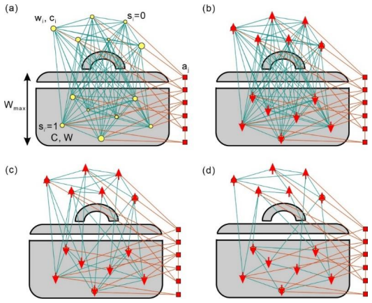
The load-bearing object is the absolute minimum core (AMC) model, a minimal two-layer grid of spins with nearest-neighbor interactions and frustrations that is supposed to retain the full hardness of the 3D spin-glass Ising model. Its brute-force cost $C_U(M_{AMC,SGI}^{3D})$ is identified with the lower bound $C_L(M_{SGI}^{3D})$, and Eq (20) asserts the same core model bounds the knapsack problem: $C_L(M_{KP}^{3D}) = C_L(M_{SGI}^{3D})$. The transfer-matrix representation supplies the topological reason: a 3D lattice mapped onto 2D transfer matrices produces crossings and interaction terms $s'_j s'_{j+mn}$ that act as long-range entanglements, and the AMC is the smallest arrangement that keeps those entanglements.
What would settle it
For a small instance, encode the knapsack Hamiltonian (14), solve its all-to-all ground state exactly, then solve the ground state of the truncated six-neighbor 3D lattice obtained by neglecting long-range couplings; any instance where the optimal assignment differs refutes the equality in Eq (20).
Extended reading notes
Core claim
The paper's central claim is Theorem 1: the lower bound of the computational complexity of the 0-1 knapsack problem on a 3D lattice, $C_L(M_{KP}^{3D})$, is subexponential and superpolynomial. Concretely, the author derives $C_L(M_{KP}^{3D}) \geq C_U(M_{AMC,KP}^{3D})$, and via Eq (20) sets this equal to the 3D spin-glass Ising lower bound $C_L(M_{SGI}^{3D})$, which is $O(2^{N^{2/3}})=O((1+\varepsilon)^N)$ with $\varepsilon \to 0$ and $\varepsilon \neq 1/N$. The same argument places an NP-intermediate (NPI) region between NP-complete and P for knapsack, with the absolute minimum core (AMC) model on the border, meaning the core cannot collapse directly into P.
Load-bearing premise
The argument stands or falls on the claim that the knapsack problem's lower bound equals the 3D spin-glass model's lower bound, a claim reached by dropping long-range couplings—and dropping couplings can only make a problem easier, so the truncated model cannot force a lower bound on the original.
Editorial extensions
If this is right
- Exact algorithms for 0-1 knapsack cannot be polynomial unless the claimed lower bound fails; the best possible running time would be $O((1+\varepsilon)^N)$ with $\varepsilon \to 0$, far below the $O(1.3^N)$ brute-force scale.
- The same subexponential, superpolynomial lower-bound class would transfer to other NP-complete problems, including TSP, K-SAT, and neural networks, through the paper's universality argument.
- The AMC model becomes a concrete target for algorithm design: solve the two-layer core by brute force and parallelize the remaining layers.
- An NP-intermediate area for knapsack exists, with incomplete AMC models playing the role of the classically constructed NP-intermediate problems.
Reading between the lines
- A direct test of the truncation step on small instances would show whether the all-to-all knapsack Hamiltonian and the six-neighbor 3D lattice share the same ground states; if not, the stated lower bound belongs only to the truncated model, not to the original knapsack problem.
- Taken literally, the phase diagram implies every NP-complete problem has a hardness core of size $N^{2/3}$, suggesting a general design principle: identify and brute-force the core, then layer the rest.
- The promised speedup from $O(1.3^N)$ to $O((1+\varepsilon)^N)$ is a concrete, benchmarkable claim; comparing the proposed layered algorithm against dynamic programming on difficult knapsack instances would quantify how close the strategy comes to the bound.
Editorial analysis
A structured set of objections, weighed in public.
Referee Report
Summary. The manuscript claims to determine a lower bound on the computational complexity of 0-1 knapsack problems, arguing that it is subexponential and superpolynomial. The argument proceeds by mapping the knapsack problem to an all-to-all (Sherrington-Kirkpatrick) Ising model, then reducing that model to a three-dimensional Edwards-Anderson model by deleting long-range interactions, and finally asserting that the lower bound of the 3D spin-glass Ising model transfers to the knapsack problem via Eq. (20). The paper also asserts the existence of an absolute minimum core (AMC) model whose brute-force complexity is declared to be a lower bound, and uses this to claim an NP-intermediate area for knapsack problems.
Significance. If correct, the result would be a striking complexity-theoretic claim: a nontrivial lower bound for a classical NP-complete optimization problem derived from statistical-mechanical reasoning. The paper does cite known NP-completeness results for spin glasses and knapsack, and it attempts to connect physical topology to complexity classes. However, the central derivation is not supported by the arguments presented. The key transfer of a lower bound from a nearest-neighbor model to an all-to-all model proceeds in the wrong direction, and the asserted lower bound itself rests on an unproved inequality from prior work. Since the main claim is load-bearing and appears unsound, the paper does not meet the standards for publication in its current form.
major comments (3)
- [Section 3.4, Eq. (20)] Equation (20) is the central identity: CL(MKP3D) = CL(MSGI3D). But the mapping in Eqs. (14)-(15) produces an all-to-all (Sherrington-Kirkpatrick) Ising Hamiltonian on N+Wmax spin variables, not a 3D nearest-neighbor Edwards-Anderson model. The proof then says the SK model can be reduced to the EA model by 'simplify neglecting the long-range interactions.' This is the wrong direction for a lower-bound transfer: deleting interactions is a relaxation that can only make the problem easier, so a lower bound on the relaxed nearest-neighbor model does not imply a lower bound on the original all-to-all model. To transfer hardness one would need a polynomial-time reduction from hard 3D EA instances to knapsack instances, which is not provided. Equations (16)-(17) only assert an ordering C(EA) < C(SK), which is not a reduction and is used backwards. Thus Theorem 1 does not follow.
- [Section 2.3, Eq. (8) and Section 3.4, Eq. (19)] The lower-bound equations (8) and (19) state that the brute-force complexity CU of the AMC model is a lower bound for the full model's complexity. This is asserted with 'It has been proven [14,15]' but no proof is given here or in the supplied manuscript. CU is, by definition, the cost of one particular algorithm (brute-force search); unless it is proven that no faster algorithm exists, CU is an upper bound on that algorithm's cost, not a lower bound for the problem. The entire chain of reasoning inherits this unsupported premise. A rigorous lower bound would require a complexity-theoretic argument, not a declaration that a hand-constructed 'core' model is minimal.
- [Section 3.4 and Section 3.5] The claimed complexity classification is stated as CL(MKP3D) in O((1+ε)^N) with ε→0 and ε≠1/N. This expression is not a well-defined complexity class: O((1+ε)^N) for variable ε is meaningless without specifying how ε scales with N, and the assertion that this equals O(2^{N^{2/3}}) is inconsistent. Moreover, the existence of NPI problems and the location of the AMC model 'on the border' are asserted without a proof that the problems under consideration are indeed neither in P nor NP-complete; Ladner's theorem gives NPI problems under P≠NP, but the paper does not establish that the constructed 'incomplete AMC models' are in NP and not in P.
minor comments (4)
- [Abstract and Section 1] The abstract mentions 'improved greatly from O(1.3N) to O((1 + ε)N)' but the standard notation for exponential time is O(1.3^N); as written it appears to claim a polynomial improvement. Please clarify.
- [Section 2.4, Eq. (10)] The chain of inequalities in Eq. (10) mixes asymptotic notation with specific functions and does not define the variable P in O(N^P); this should be written with explicit complexity classes or growth rates.
- [Section 3.1, Definitions] Definitions 6 and 7 introduce many symbols (MKPall, MKP3D, MKP2D, MAMC,KP3D, etc.) that are used inconsistently; for example, the proof of Theorem 1 sometimes writes CL(MKP3D) and sometimes CL(MSGI3D) without clarifying the relationship between these models beyond Eq. (20).
- [Figures] Figures 1, 2, 4, 5, 6, and 7 are described but not displayed in the text; their content is essential for interpreting the AMC model and the alleged topological crossings. Please ensure the figures are included and legible.
Circularity Check
The claimed knapsack lower bound is the same author's prior spin-glass lower bound, imported by self-citation (Eq. 8) and equated by assertion (Eq. 20); Theorem 1 restates Eq. 20 rather than deriving it.
-
self citation load bearing
[Section 2.3, Eq. (8)]
"It has been proven [14,15] that for the 3D spin-glass Ising model, the upper bound of the complexity (by brute force search) of the AMC model gives its lower bound. That is, CL(MSGI3D) ≥ CU(MAMC,SGI3D). (8)"
The lower bound that the paper transfers to the knapsack problem is not derived here; it is imported from the same author's earlier papers [14,15]. Defining CU as a brute-force upper bound and then declaring it to be a lower bound is precisely the claim that no faster algorithm for the AMC model exists, which is the desired lower-bound statement. The only justification offered is 'Theorem 2 in [14]', another same-author result asserting that no algorithm can break the global entanglements of the AMC model. No machine-checked proof, external benchmark, or independent parameter-free derivation is supplied, so the central lower bound is an input, not a conclusion.
-
renaming known result
[Section 3.4, Eq. (20)]
"By adjusting/removing the unimportant weights in the knapsacks, one may disconnect some long-range interactions between spins, to obtain an 'easier' arrangement of spins with only the nearest interaction in the 3D lattice. ... I have CL(MKP3D) = CL(MSGI3D) ≥ CU(MAMC,SGI3D) = CU(MAMC,KP3D). (20)"
Eq. (20) is the proof's load-bearing step and it simply equates the knapsack lower bound with the already-imported spin-glass lower bound. The knapsack mapping in Eqs. (14)-(15) produces an all-to-all Ising model, so 'adjusting/removing weights' to reach a nearest-neighbour 3D lattice is a relaxation; a lower bound on the relaxed model does not transfer to the original problem. The paper has no polynomial-time embedding of arbitrary 3D spin-glass instances into knapsack instances. Consequently Theorem 1's subexponential-superpolynomial bound is just the prior CL(MSGI3D) value renamed as CL(MKP3D) via Eq. (20), which is circular by construction.
1 more flagged steps
-
uniqueness imported from authors
[Section 2.3, paragraph before Eq. (8)]
"According to Theorem 2 in [14], to find the exact solution of the 3D spin-glass Ising model, any algorithms cannot break the global effects of entanglements in the AMC model."
This self-cited 'Theorem 2' is what turns the brute-force count CU(MAMC,SGI3D) into a universal lower bound: it asserts that every algorithm must pay the full AMC entanglement cost. The theorem is imported from the same author's prior work [14] and is not re-proved or independently verified in this paper. It is used as an external mathematical fact to rule out all faster algorithms, which is the pattern of uniqueness imported from the authors rather than derived.
full rationale
The paper's positive content — the Hamiltonian mapping from the 0-1 knapsack problem to an all-to-all Ising model, Eqs. (14)-(15) — is standard and taken from Kyriienko et al. [39]; that part is not circular. However, the claimed lower bound is not obtained from this mapping. Theorem 1 depends on Eq. (20), which asserts CL(MKP3D)=CL(MSGI3D), and on Eq. (8), which asserts CL(MSGI3D)≥CU(MAMC,SGI3D) by reference to the author's [14,15]. The latter statement identifies a brute-force upper bound of a hand-constructed AMC submodel with a lower bound; the only support is the author's own 'Theorem 2 in [14]'. The proof then transfers this value to the knapsack problem by removing/adjusting weights to reach a nearest-neighbour lattice, which is the wrong direction for a lower-bound argument. Eqs. (16)-(17) compare complexities of SK and EA models but do not supply a reduction from hard spin-glass instances to knapsack instances. Thus the central result is forced by a self-citation chain plus the asserted equality Eq. (20), not by an independent derivation. External refs. [33-35] merely 'recognized' the prior spin-glass results and are not independent benchmarks. Correctness concerns such as the relaxation direction are separate from circularity, but here they converge: the knapsack bound is the prior spin-glass bound renamed.
Assumptions & free parameters
free parameters (2)
- alpha and beta in the knapsack Hamiltonian
- z, the number of layers in the algorithm element
assumptions (6)
- standard math Cook-Levin theorem: satisfiability and related problems are NP-complete
- standard math Ladner's theorem: if P != NP, there exist NP-intermediate problems
- domain assumption The mapping between 0-1 knapsack and all-to-all Ising model given by Eqs (14)-(15) faithfully represents the knapsack optimum
- ad hoc to paper From [14,15]: CL(MSGI3D) >= CU(MAMC,SGI3D), the brute-force complexity of the AMC model is a lower bound for the full model
- ad hoc to paper Cutting long-range interactions reduces the Sherrington-Kirkpatrick model to the 3D Edwards-Anderson model while preserving hardness relations
- ad hoc to paper CL(MKP3D) = CL(MSGI3D)
invented entities (3)
-
3D knapsack problem MKP3D
-
AMC model for knapsack MAMC,KP3D
-
NPI problem for knapsack MNPI,KP
Cite this review
Pith. "Pith review of Lower bound of computational complexity of knapsack problems." pith.science (2026). https://pith.science/paper/75L722YZ
@misc{pith2026250612080,
  author       = {Pith},
  title        = {Pith review of: Lower bound of computational complexity of knapsack problems},
  year         = {2026},
  howpublished = {\url{https://pith.science/paper/75L722YZ}},
  note         = {Machine review of arXiv:2506.12080}
}
read the original abstract
The quantum statistics mechanism is very powerful for investigating the equilibrium states and the phase transitions in complex spin disorder systems. The spin disorder systems act as an interdisciplinary platform for solving the optimum processes in computer science. In this work, I determined the lower bound of the computational complexity of knapsack problems. I investigated the origin of nontrivial topological structures in these hard problems. It was uncovered that the nontrivial topological structures arise from the contradictory between the three-dimensional character of the lattice and the two-dimensional character of the transfer matrices used in the quantum statistics mechanism. I illustrated a phase diagram for the non-deterministic polynomial (NP) vs polynomial (P) problems, in which a NP-intermediate (NPI) area exists between the NP-complete problems and the P-problems, while the absolute minimum core model is at the border between the NPI and the NP-complete problems. The absolute minimum core model of the knapsack problem cannot collapse directly into the P-problem. Under the guide of the results, one may develop the best algorithms for solving various optimum problems in the shortest time, being in subexponential and superpolynomial. This work illuminates the road on various fields of science ranging from physics to biology to finances, and to information technologies.
Figures


Figures from the paper (4 more)


Reference graph
Works this paper leans on
-
[1]
Huang, Statistical mechanics, New York: Wiley, 2008
K. Huang, Statistical mechanics, New York: Wiley, 2008
work page 2008
-
[2]
C. P. Bachas, Computer-intractability of the frustration model of a spin glass, J. Phys. A: Math. Gen. , 17 (1984), L709. https://doi.org/10.1088/0305- 4470/17/13/006
doi:10.1088/0305- 1984
-
[3]
Barahona, On the computational complexity of Ising spin glass models, J
F. Barahona, On the computational complexity of Ising spin glass models, J. Phys. A: Math. Gen., 15 (1982), 3241. https://doi.org/10.1088/0305-4470/15/10/028
-
[4]
S. F. Edwards, P. W. Anderson, Theory of spin glasses, J. Phys. F: Met. Phys., 5 (1975), 965–974. https://doi.org/10.1088/0305-4608/5/5/017
-
[5]
Istrail , Statistical mechanics, three -dimensionality and NP -completeness: I
S. Istrail , Statistical mechanics, three -dimensionality and NP -completeness: I. Universality of intracatability for the partition function of the Ising model across non-planar surfaces (extended abstract), Proceedings of the thirty -second annual ACM symposium on The ory of computing , 2000, 87 –96. https://doi.org/10.1145/335305.335316
-
[6]
D. L. Stein, C. M. Newman, Spin Glasses and Complexity , Princeton University Press, 2013
work page 2013
-
[7]
Ising, Beitrag zur theorie des ferromagnetismus, Z
E. Ising, Beitrag zur theorie des ferromagnetismus, Z. Phys., 31 (1925), 253–258. https://doi.org/10.1007/BF02980577
-
[8]
Onsager, Crystal statistics I: a two -dimensional model with an order -disorder transition, Phys
L. Onsager, Crystal statistics I: a two -dimensional model with an order -disorder transition, Phys. Rev. , 65 (1944), 117 –149. https://doi.org/10.1103/PhysRev.65.117
Show all 59 references
-
[9]
Z. D. Zhang, Conjectures on the exact solution of three -dimensional (3D) simple orthorhombic Ising lattices, Phil. Mag. , 87 (2007), 5309 –5419. https://doi.org/10.1080/14786430701646325
2007 doi
-
[10]
Garey, D
M. Garey, D. S. Johnson, Computers and intractability, A guide to the Theory of NP-completeness, W. H. Freeman and Company, San Francisco, 1979
1979
-
[11]
C. H. Papadimitriou, Computational Complexity, Addison-Wesley, 1994
1994
-
[12]
Cook, The complexity of theorem-proving procedures, Proceedings of the third annual ACM symposium on Theory of computing , 1971, 151 –158
S. Cook, The complexity of theorem-proving procedures, Proceedings of the third annual ACM symposium on Theory of computing , 1971, 151 –158. https://doi.org/10.1145/800157.805047
1971
-
[13]
L. A. Levin, Universal sequential search problems, Probl. Inform. Transm. , 9 (1973), 265-266
1973
-
[14]
Z. D. Zhang, Computational complexity of spin-glass three-dimensional (3D) Ising model, J. Mater. Sci. Tech. , 44 (2020), 116 –120. https://doi.org/10.1016/j.jmst.2019.12.009
2020 doi
-
[15]
Z. D. Zhang, Mapping between spin-glass three-dimensional (3D) Ising model and Boolean satisfiability problem, Mathematics, 11 (2023), 237. https://doi.org/10.3390/math11010237
2023 doi
-
[16]
Dantzig, Numbers: the language of science, London: George Allen & Unwin, Ltd., 1930
T. Dantzig, Numbers: the language of science, London: George Allen & Unwin, Ltd., 1930
1930
-
[17]
G. B. Mathews, On the partition of numbers, Proc. London Math. Soc., 28 (1897), 486–490. https://doi.org/10.1112/plms/s1-28.1.486
-
[18]
Mar tello, D
S. Mar tello, D. Pisinger, P. Toth, New trends in exact algorithms for the 0 -1 knapsack problem, Eur. J. Oper. Res. , 123 (2000), 325 –332. https://doi.org/10.1016/S0377-2217(99)00260-X
2000 doi
-
[19]
Pisinger, Where are the hard knapsack problems? Comput
D. Pisinger, Where are the hard knapsack problems? Comput. Oper. Res. , 32 (2005), 2271–2284. https://doi.org/10.1016/j.cor.2004.03.002
2005 doi
-
[20]
Fayard, G
D. Fayard, G. Plateau, Resolution of the 0 -1 knapsack problem: comparison of methods, Math. Program. , 8 (1975), 272 –307. https://doi.org/10.1007/BF01580448
1975 doi
-
[22]
Al -Shihabi, A novel core -based optimization framework for binary integer programs- the multidemand multidimesional knapsack problem as a test problem, Oper
S. Al -Shihabi, A novel core -based optimization framework for binary integer programs- the multidemand multidimesional knapsack problem as a test problem, Oper. Res. Perspect., 8 (2021), 100182. https://doi.org/10.1016/j.orp.2021.100182
2021
-
[23]
D. E. Armstrong, S. H. Jacobson, Data -independent neighborhood functions and strict local optima, Discrete Appl. Math. , 146 (2005), 233 –243. https://doi.org/10.1016/j.dam.2004.09.007
2005 doi
-
[24]
D. S. Johnson, Approximation algorithms for combinatorial problems, J. Comput. Syst. Sci., 9 (1974), 256–278. https://doi.org/10.1016/S0022-0000(74)80044-9
1974 doi
-
[25]
Toth, Optimization enginee ring techniques for the exact solution of NP -hard combinatorial optimization problems, Eur
P. Toth, Optimization enginee ring techniques for the exact solution of NP -hard combinatorial optimization problems, Eur. J. Oper. Res. , 125 (2000), 222 –238. https://doi.org/10.1016/S0377-2217(99)00453-1
2000 doi
-
[26]
Venkataraman, G
G. Venkataraman, G. Athithan, Spin glass, the travelling salesman problem, neural networks and all that, Pramana-J. Phys. , 36 (1991), 1 –77. https://doi.org/10.1007/BF02846491
1991 doi
-
[27]
Z. D. Zhang, O. Suzuki, N. H. March, Clifford algebra approach of 3D Ising model, Adv. Appl. Clifford Algebras, 29 (2019), 12. https://doi.org/10.1007/s00006-018- 0923-2
2019 doi
-
[28]
Suzuki, Z
O. Suzuki, Z. D. Zhang, A method of Riemann -Hilbert problem for Zhang ’s conjecture 1 in a ferromagnetic 3D Ising model: trivialization of topological structure, Mathematics, 9 (2021), 776. https://doi.org/10.3390/math9070776
2021 doi
-
[29]
B.C. Li, W. Wang, Exploration of dynamic phase transition of 3D Ising model with a new long-range interaction by using the Monte Carlo Method, Chin. J. Phys., 90 (2024), 15–30. https://doi.org/10.1016/j.cjph.2024.05.021
2024 doi
-
[30]
Ghosh, C
K. Ghosh, C. J. Lobb, R. L. Greene, Critical phenomena in the double -exchange ferromagnet La 0.7Sr0.3MnO3, Phys. Rev. Lett. , 81 (1998), 4740 –4743. https://doi.org/10.1103/PhysRevLett.81.4740
1998 doi
-
[31]
J. T. Ho, J. D. Litster, Magnetic equation of state of CrBr 3 near the critical point, Phys. Rev. Lett., 22 (1969), 603–606. https://doi.org/10.1103/PhysRevLett.22.603
1969 doi
-
[32]
Y . Liu, V . N. Ivanovski, C. Petrovic, Critical behavior of the van der Waals bonded ferromagnet Fe 3−xGeTe2, Phys. Rev. B , 96 (2017), 144429. https://doi.org/10.1103/PhysRevB.96.144429
2017 doi
-
[33]
F. X. Liu, L. M. Duan, Computational characteristics of the random -field Ising model with long -range interaction, P hys. Rev. A , 108 (2023), 0124 15. https://doi.org/10.1103/PhysRevA.108.012415
2023 doi
-
[34]
S. Nagy, R. Paredes, J. M. Dudek, L. Dueñ as-Osorio, M. Y. Vardi, Ising model partition-function computation as a weighted counting problem, Phys. Rev. E, 109 (2024), 055301. https://doi.org/10.1103/PhysRevE.109.055301
2024 doi
-
[35]
H. J. Xu, S. Dasgupta, A. Pothen , A. Banerjee, Dynamic asset allocation with expected shortfall via quantum annealing, Entropy, 25 (2023), 541. https://doi.org/10.3390/e25030541
2023 doi
-
[36]
Ladner, On the structure of polynomial time r educibility, J
R. Ladner, On the structure of polynomial time r educibility, J. ACM, 22 (1975), 155–171. https://doi.org/10.1145/321864.321877
1975
-
[37]
Jonsson, V
P. Jonsson, V . Lagerkvist, G. Nordh, Constructing NP -intermediate problems by blowing holes with parameters of various properties, Theor. Comput. Sci. , 581 (2015), 67–82. https://doi.org/10.1016/j.tcs.2015.03.009
2015 doi
-
[38]
Bellman, A Markovian decision process, J
R. Bellman, A Markovian decision process, J. Math. Mech. , 6 (1957), 679–684. https://doi.org/10.1512/iumj.1957.6.56038
1957 doi
-
[39]
Kyriienko, H
O. Kyriienko, H. Sigurdsson, T. C. H. Liew, Probabilistic solving o f NP-hard problems with bistable nonlinear optical networks, Phys. Rev. B , 99 (2019), 195301. https://doi.org/10.1103/PhysRevB.99.195301
2019 doi
-
[40]
G. B. Dantzig, Discrete-variable extremum problems, Oper. Res., 5 (1957), 161–
1957
-
[41]
Bellman, Letter to the Editor–Comment on Dantzig’s paper on discrete-variable extremum problems, Oper
R. Bellman, Letter to the Editor–Comment on Dantzig’s paper on discrete-variable extremum problems, Oper. Res. , 5 (1957), 613 –738. https://doi.org/10.1287/opre.5.5.723
1957 doi
-
[43]
Cacchiani, M
V. Cacchiani, M. Iori, A. Locatelli, S. Martello, Knapsack problems–an overview of recent advances. Part II: Multiple, multidimensional, and quadratic knapsack problems, Comput. Oper. Res. , 143 (2022), 105693. https://doi.org/10.1016/j.cor.2021.105693
2022
-
[44]
Kellerer, U
H. Kellerer, U. Pferschy, D. Pisinger, Knapsack problems, Springer-Verlag, 2004. https://doi.org/10.1007/978-3-540-24777-7
2004 doi
-
[45]
Nishimori, Statistical physics of spin glasses and information processing: an introduction, Oxford University Press, 2001
H. Nishimori, Statistical physics of spin glasses and information processing: an introduction, Oxford University Press, 2001
2001
-
[46]
Kirkpatrick, D
S. Kirkpatrick, D. Sherrington, Infinite-ranged models of spin-glasses, Phys. Rev. B, 17 (1978), 4384–4403. https://doi.org/10.1103/PhysRevB.17.4384
1978 doi
-
[47]
Sherrington, S
D. Sherrington, S. Kirkpatrick, Solvable model of a spin-glass, Phys. Rev. Lett., 35 (1975), 1792–1796. https://doi.org/10.1103/PhysRevLett.35.1792
1975 doi
-
[48]
Boccaletti, V
S. Boccaletti, V. Latora, Y. Moreno, M. Chavez, D. U. Hwang, Complex networks: structure and dynamics, Phys. Rep. , 424 (2006), 175 –308. https://doi.org/10.1016/j.physrep.2005.10.009
2006 doi
-
[49]
G. E. Hinton, R. R. Salakhutdinov, Reducing the dimensionality of data with neural networks, Science, 313 (2006), 504 –507. https://doi.org/10.1126/science.1127647
2006 doi
-
[50]
M. K. Kwan, Graphic programming using odd or even points, Chin. Math., 1 (1962), 273–277
1962
-
[51]
U. U. Haus, K. Niermann, K. Truemper, R. Weismantel, Logic integer programming models for signaling networks, J. Comput. Biol. , 16 (2009), 725–
2009
-
[52]
Bertsimas , R
D. Bertsimas , R. Demir , An approximate dynamic programming approach to multidimensional Knapsack problems , Manag. Sci. , 48 (2002), 453–590. https://doi.org/10.1287/mnsc.48.4.550.208
2002 doi
-
[53]
G. J. Woeginger, When does a dynamic programming formulation guarantee the existence of a fully polynomial time approximation scheme (FPTAS)? J. Comput., 12 (2000), 1–82. https://doi.org/10.1287/ijoc.12.1.57.11901
2000 doi
-
[54]
Balas, N
E. Balas, N . Simonetti, Linear time dynamic-programming algorithms for new classes of restricted TSPs: a computational study, J. Comput., 13 (2001), 1–94. https://doi.org/10.1287/ijoc.13.1.56.9748
2001 doi
-
[55]
A. A. Melkman, T. Akutsu, An improved satisfiability algorithm for nested canalyzing functions and its application to determining a singleton attractor of a Boolean network, J. Comput. Biol. , 20 (2013), 958 –969. https://doi.org/10.1089/cmb.2013.0060
2013
-
[56]
P. C. Chu, J. E. Beasley, A genetic algorithm for the multidimensional Knapsack problem, J. Heuristics , 4 (1998), 63 –86. https://doi.org/10.1023/A:1009642405419
1998 doi
-
[57]
A. K. Hartmann, Ground-state behavior of the three-dimensional J random-bond Ising model, Phys. Rev. B , 59 (1999), 3617. https://doi.org/10.1103/PhysRevB.59.3617
1999 doi
-
[58]
L. V. Snyder, M. S. Daskin , A random-key genetic algorithm for the generalized traveling salesman problem, Eur. J. Oper. Res. , 174 (2006), 38 –53. https://doi.org/10.1016/j.ejor.2004.09.057
2006 doi
-
[59]
Larranaga, C
P. Larranaga, C. M. H. Kuijpers, R. H. Murga, I. Inza, S. Dizdarevic, Genetic algorithms for the travelling salesman problem: A review of representations and operators, Artif. Intell. Rev. , 13 (1999), 129 –170. https://doi.org/10.1023/A:1006529012972
1999 doi
-
[306]
https://doi.org/10.1287/opre.5.2.266
-
[743]
https://doi.org/10.1089/cmb.2008.0163
2008
Reviewed August 7, 2026 · model on record in the stance chip above.
Discussion (0). Sign in to comment.