Machine-Learning-Powered Specification Testing in Linear Instrumental Variable Models

Cyrill Scheidegger; Malte Londschien; Peter B\"uhlmann

arxiv: 2506.12771 · v3 · submitted 2025-06-15 · 📊 stat.ME

Machine-Learning-Powered Specification Testing in Linear Instrumental Variable Models

Cyrill Scheidegger , Malte Londschien , Peter B\"uhlmann This is my paper

Pith reviewed 2026-05-19 09:43 UTC · model grok-4.3

classification 📊 stat.ME

keywords instrumental variablesspecification testingmachine learningresidual predictionjust-identified modelsmean independence

0 comments

The pith

A residual-prediction test powered by machine learning checks linear IV model specification under mean independence of the structural error from the instruments.

A machine-rendered reading of the paper's core claim, the machinery that carries it, and where it could break.

The paper develops a test for whether a linear IV model is correctly specified by checking if the two-stage least squares residuals can be predicted from the instruments using a machine learning method. This approach works under the assumption that the structural error is mean independent of the instruments, which permits testing even when the number of instruments equals the number of endogenous variables. The test uses sample splitting to achieve asymptotic control of the type I error rate and demonstrates consistency against many alternatives. It also extends to cases with weak or numerous instruments through an inversion similar to the Anderson-Rubin test and supports robust standard errors for heteroskedasticity and clustering.

Core claim

Under the mean independence of the structural error from the instruments, the linear IV model is well-specified if and only if the 2SLS residuals are unpredictable from the instruments. The proposed test implements this idea by training a machine learning predictor on a sample split and testing whether its out-of-sample prediction error is better than a null benchmark, yielding a valid p-value that controls type I error asymptotically and has power against misspecifications where the residuals carry information about the instruments.

What carries the argument

The residual prediction test, which assesses whether two-stage least squares residuals are predictable from the instruments using sample splitting and an arbitrary machine learning method.

If this is right

The test applies directly to just-identified IV models where classical overidentification tests cannot be used.
It maintains validity under heteroskedasticity and clustering through appropriate variance estimators.
The method extends to weak instrument settings by inverting an Anderson-Rubin-type statistic.
Consistency holds against a broad class of alternatives where the structural error depends on the instruments.

Where Pith is reading between the lines

These are editorial extensions of the paper, not claims the author makes directly.

This test can be applied in many empirical studies that rely on exactly identified IV designs.
The approach opens the door to using more flexible predictors to increase detection power for subtle misspecifications.
Similar residual-based testing ideas could be explored in other econometric models with endogeneity corrections.

Load-bearing premise

The structural error term is mean independent of the instruments.

What would settle it

If repeated applications of the test to data generated from a correctly specified linear IV model reject the null hypothesis at rates exceeding the nominal level, the asymptotic type I error control would be falsified.

Figures

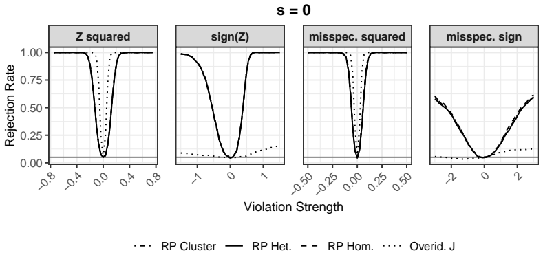
Figures reproduced from arXiv: 2506.12771 by Cyrill Scheidegger, Malte Londschien, Peter B\"uhlmann.

**Figure 1.** Figure 1: Simulation results under H0 under the four data generating processes. The black solid line is the rejection rate using RP Het., the black dashed line using RP Hom., and the black dotted line using Overid. J. The gray solid line indicates the significane level α = 0.05 and the gray dashed lines indicate (pointwise) 95%-test bounds for the rejection rates, that is: if the level of the test is indeed α = 0.05… view at source ↗

**Figure 2.** Figure 2: Simulation results under HA with the data generating process just-identified, homoskedastic with n = 400. The black solid line is the rejection rate using RP Het., the black dashed line using RP Hom., and the black dotted line using Overid. J. When the black dashed line is not visible, it is identical to the black solid line. The gray solid line indicates the significance level α = 0.05. Additional simula… view at source ↗

**Figure 3.** Figure 3: Simulation results under HA with the data generating process overidentified, homoskedastic with n = 400. The black solid line is the rejection rate using RP Het., the black dashed line using RP Hom., and the black dotted line using Overid. J. When the black dashed line is not visible, it is identical to the black solid line. The gray solid line indicates the significance level α = 0.05. demographic dummy … view at source ↗

**Figure 4.** Figure 4: Simulation results under H0 with clustered dependence structure (cluster size 4) in the setting just-identified, homoskedastic for n ∈ {100, 200, 400, 800} and varying strength s ∈ [0, 1] of cluster dependency. The black dash-dotted line is the rejection rate using RP Cluster, the black solid line is the rejection rate using RP Het., the black dashed line using RP Hom., and the black dotted line using Over… view at source ↗

**Figure 5.** Figure 5: Simulation results under HA in the setting just-identified, homoskedastic for n = 400 and s = 0 (i.i.d. data). The black dash-dotted line is the rejection rate using RP Cluster, the black solid line is the rejection rate using RP Het., the black dashed line using RP Hom., and the black dotted line using Overid. J. When the dashed or the dash-dotted line is not visible, it is identical to the solid line. Th… view at source ↗

**Figure 6.** Figure 6: Simulation results under HA in the setting just-identified, homoskedastic for n = 400 clustered dependency structure (cluster size 4) with s = 0.8. The black dash-dotted line is the rejection rate using RP Cluster, the black solid line is the rejection rate using RP Het., the black dashed line using RP Hom., and the black dotted line using Overid. J. When the dashed line is not visible, it is identical to … view at source ↗

**Figure 7.** Figure 7: Simulation results under HA with the data generating process just-identified, heteroskedastic with n = 400. The black solid line is the rejection rate using RP Het., the black dashed line using RP Hom., and the black dotted line using Overid. J. The gray solid line indicates the significance level α = 0.05. Z squared sign(Z) misspec. squared misspec. sign −0.8 −0.4 0.0 0.4 0.8 −1 0 1 −0.50 −0.25 0.00 0.25… view at source ↗

**Figure 8.** Figure 8: Simulation results under HA with the data generating process overidentified, heteroskedastic with n = 400. The black solid line is the rejection rate using RP Het., the black dashed line using RP Hom., and the black dotted line using Overid. J. The gray solid line indicates the significance level α = 0.05. 42 [PITH_FULL_IMAGE:figures/full_fig_p042_8.png] view at source ↗

read the original abstract

The linear instrumental variable (IV) model is widely used in observational studies, yet its validity hinges on strong assumptions. Classical specification tests such as the Sargan-Hansen J test are limited to overidentified settings and are therefore not applicable in the common just-identified case, where the number of instruments is equal to the number of endogenous variables. We propose a novel test for the well-specification of the linear IV model under the assumption that the structural error is mean independent of the instruments. This assumption enables specification testing even in the just-identified setting. Our approach uses the idea of residual prediction: if the two-stage least squares residuals can be predicted from the instruments better than chance, this indicates misspecification. The resulting test employs sample splitting and a user-chosen machine learning method, and we show asymptotic type I error control and consistency against a broad class of alternatives. We further show how the proposed testing principle can be adapted to settings with weak or many instruments via an Anderson-Rubin-type inversion, thereby substantially extending the applicability. The tests accommodate heteroskedasticity- and cluster-robust inference and are implemented in the R package RPIV and the ivmodels software package for Python.

Editorial analysis

A structured set of objections, weighed in public.

Desk editor's note, referee report, simulated authors' rebuttal, and a circularity audit. Tearing a paper down is the easy half of reading it; the pith above is the substance, this is the friction.

Desk Editor's Note private letter to a colleague

This paper gives a usable specification test for linear IV models in the just-identified case by checking whether 2SLS residuals can be predicted from the instruments via ML after sample splitting.

read the letter

The main contribution is a residual-prediction test that lets you check the linear IV model even when instruments equal endogenous regressors. Under mean independence of the structural error from the instruments, the 2SLS residuals should not be predictable from Z better than chance. They turn this into a test statistic with sample splitting and any user-chosen ML method, then prove asymptotic type I error control and consistency against broad alternatives. They also adapt the same idea to weak instruments through an Anderson-Rubin inversion, which keeps the orthogonality intact and extends the reach quite a bit. That combination is new relative to the classical Sargan-Hansen test, which simply does not apply in the just-identified setting that is common in practice. The paper handles heteroskedasticity and clustering, and the authors supply R and Python packages, which is helpful for adoption. The asymptotic claims look internally consistent with the construction described, and sample splitting removes the usual overfitting worry with ML. The central assumption is stated clearly and is weaker than what overidentification tests require. One soft spot is that the exact regularity conditions for the ML step and the rate at which the prediction error vanishes are not visible from the abstract alone, so the proofs will need a close read to confirm they cover typical ML estimators without extra restrictions. Finite-sample behavior will also depend on the chosen ML method, even if the theory is broad. This is aimed at applied econometricians and causal-inference researchers who run just-identified or weakly identified IV models and want a specification check where none existed before. A reader working on empirical applications with observational data would get direct value from the method and the software. The work is coherent on its own terms and targets a real gap, so it deserves a serious referee.

Referee Report

2 major / 3 minor

Summary. The paper proposes a residual-prediction test for specification of linear IV models under the mean independence of structural errors and instruments. This enables testing in the just-identified case (where Sargan-Hansen does not apply) by checking whether 2SLS residuals can be predicted from instruments better than chance, using sample splitting and a user-chosen ML method. Asymptotic type I error control and consistency against broad alternatives are claimed, along with an Anderson-Rubin-style inversion extension for weak or many instruments that preserves the orthogonality principle; the tests allow heteroskedasticity- and cluster-robust inference and are implemented in R and Python packages.

Significance. If the asymptotic results hold, the contribution is meaningful: it fills a practical gap by providing a specification test for the common just-identified IV setting and flexibly incorporates modern ML while retaining valid inference. The AR inversion broadens applicability to weak-instrument regimes. Explicit software implementations and the focus on falsifiable prediction-based diagnostics are strengths that could make the method adoptable in applied work.

major comments (2)

[§3.1, Theorem 1] §3.1, Theorem 1: the claimed asymptotic normality of the test statistic after robust variance estimation requires explicit rate conditions on the ML predictor (e.g., o_p(n^{-1/4}) uniform convergence of the fitted residuals); without these, the orthogonality argument used to separate estimation error from the prediction step may not go through under the stated mean-independence null.
[§4.2, Algorithm 2] §4.2, Algorithm 2: the Anderson-Rubin inversion is described at a high level, but the paper does not specify how the critical value or the grid search is adjusted when the underlying test statistic is itself ML-based; this leaves open whether the inversion preserves exact finite-sample size or only asymptotic validity under weak instruments.

minor comments (3)

The abstract and introduction should cite the precise regularity conditions under which the ML method is allowed (e.g., whether random forests, neural nets, or kernel methods are covered by the same theorem).
[Table 1] Table 1: the simulation design uses a fixed ML hyper-parameter grid; reporting sensitivity to that choice would strengthen the robustness claim.
[Eq. (8)] Notation: the symbol for the out-of-sample prediction error in Eq. (8) is easily confused with the in-sample residual; a clearer subscript would help.

Simulated Author's Rebuttal

2 responses · 0 unresolved

We thank the referee for the constructive and detailed comments. We address each major comment below and indicate the changes we will make to strengthen the manuscript.

read point-by-point responses

Referee: [§3.1, Theorem 1] §3.1, Theorem 1: the claimed asymptotic normality of the test statistic after robust variance estimation requires explicit rate conditions on the ML predictor (e.g., o_p(n^{-1/4}) uniform convergence of the fitted residuals); without these, the orthogonality argument used to separate estimation error from the prediction step may not go through under the stated mean-independence null.

Authors: We thank the referee for highlighting this point. Our proof of asymptotic normality for the test statistic relies on sample splitting to achieve Neyman orthogonality between the residual prediction step and the first-stage estimation error. However, to ensure the result holds after robust variance estimation, we agree that explicit rate conditions on the ML predictor are necessary. We will revise §3.1 to state an additional assumption requiring that the ML estimator satisfies o_p(n^{-1/4}) convergence in the relevant norm (uniformly over the instruments), and we will update the statement of Theorem 1 and the proof sketch in the appendix to incorporate this condition explicitly. This clarification does not change the main claims but makes the technical requirements precise. revision: yes
Referee: [§4.2, Algorithm 2] §4.2, Algorithm 2: the Anderson-Rubin inversion is described at a high level, but the paper does not specify how the critical value or the grid search is adjusted when the underlying test statistic is itself ML-based; this leaves open whether the inversion preserves exact finite-sample size or only asymptotic validity under weak instruments.

Authors: We appreciate the referee's request for greater detail. The Anderson-Rubin-style inversion is constructed to deliver asymptotic validity under weak or many instruments, inheriting the asymptotic type I error control of the underlying ML-based test; it is not designed to achieve exact finite-sample size control because of the data-dependent ML component. In the revision we will expand the description of Algorithm 2 to specify the grid-search implementation, including the use of asymptotic critical values obtained from the limiting distribution of the ML-based statistic (adjusted for the chosen significance level). We will also add an explicit remark clarifying that the procedure yields asymptotic rather than exact finite-sample validity. revision: yes

Circularity Check

0 steps flagged

No significant circularity; derivation self-contained

full rationale

The proposed residual-prediction test constructs its statistic from out-of-sample ML prediction performance on sample-split data, with asymptotic type I error control and consistency derived under the explicit mean-independence assumption. No step reduces a prediction or uniqueness claim to a fitted parameter by construction, nor does the central argument rest on self-citation chains or imported ansatzes. Standard regularity conditions and robust variance estimation support the limits without circular reduction to inputs.

Axiom & Free-Parameter Ledger

1 free parameters · 1 axioms · 0 invented entities

The central claim rests on the mean independence assumption and standard asymptotic theory for sample-split estimators; no free parameters beyond user choice of ML method and no invented entities.

free parameters (1)

Machine learning method
User-chosen ML algorithm for residual prediction; its properties affect finite-sample behavior but not the asymptotic claim.

axioms (1)

domain assumption Structural error is mean independent of the instruments
Invoked to enable testing in just-identified settings and to justify the residual prediction principle.

pith-pipeline@v0.9.0 · 5742 in / 1234 out tokens · 32429 ms · 2026-05-19T09:43:20.250629+00:00 · methodology

discussion (0)

Lean theorems connected to this paper

Citations machine-checked in the Pith Canon. Every link opens the source theorem in the public Lean library.

IndisputableMonolith/Cost/FunctionalEquation washburn_uniqueness_aczel unclear

?

unclear
Relation between the paper passage and the cited Recognition theorem.

We propose a novel test for the well-specification of the linear IV model under the assumption that the structural error is mean independent of the instruments... residual prediction: if the two-stage least squares residuals can be predicted from the instruments better than chance
IndisputableMonolith/Foundation/RealityFromDistinction reality_from_one_distinction unclear

?

unclear
Relation between the paper passage and the cited Recognition theorem.

We show asymptotic type I error control and consistency against a broad class of alternatives

What do these tags mean?

matches: The paper's claim is directly supported by a theorem in the formal canon.
supports: The theorem supports part of the paper's argument, but the paper may add assumptions or extra steps.
extends: The paper goes beyond the formal theorem; the theorem is a base layer rather than the whole result.
uses: The paper appears to rely on the theorem as machinery.
contradicts: The paper's claim conflicts with a theorem or certificate in the canon.
unclear: Pith found a possible connection, but the passage is too broad, indirect, or ambiguous to say the theorem truly supports the claim.

Reference graph

Works this paper leans on

16 extracted references · 16 canonical work pages

[1]

σmin ED,P [ZZ T ] ≥ c,

work page
[2]

ED,P [ZZ T ] op ≤ C, 4

σmin ED,P [ZX T ] ≥ c, 3. ED,P [ZZ T ] op ≤ C, 4. ED,P [ZX T ] op ≤ C,

work page
[3]

Next, we need some kind of uniform central limit theorem and law of large numbers

∥ED,P [Zϵ]∥op ≤ C. Next, we need some kind of uniform central limit theorem and law of large numbers. Assumption 6. It holds that lim n→∞ sup P ∈P sup w∈VD,P (ζ) sup t∈R PP 1 σw √n0 X i∈D (U w i − EP [U w i ]) ≤ t ! − Φ(t) = 0 with U w i = (w(Zi) + AT wZi)ϵi. Due to the boundedness of w, this assumption can often be motivated using the Lindeberg-Feller ce...

work page 2019
[4]

√n0∥ˆED[Zϵ] − ED,P [Zϵ]∥2 = OP(1),

work page
[5]

∥ˆED[XZ T ] − ED,P [XZ T ]∥op = oP(1), 24

work page
[6]

∥ˆED[ZZ T ] − ED,P [ZZ T ]∥op = oP(1),

work page
[7]

Finally, we also need a consistent estimator for the asymptotic variance σ2 w

∥ˆED[w(Z)X] − ED,P [w(Z)X]∥2 = oP,W(1). Finally, we also need a consistent estimator for the asymptotic variance σ2 w. Assumption 8. We have an estimator ˆσ2 w of σ2 w that satisfies σ2 w − ˆσ2 w = oP,W(1). Under Assumptions 5, 6, 7 and 8, we have uniform asymptotic normality of the test statistic 1√n0ˆσw P i∈D w(Zi) ˆRi. Theorem 6. Let N(w) be defined in...

work page
[8]

EP [∥Zi∥2+η 2 |ϵi|2+η] ≤ C,

work page
[9]

EP [∥Zi∥2+η 2 ] ≤ C,

work page
[10]

EP [∥Xi∥2 2∥Zi∥2 2] < C ,

work page
[11]

Proposition 7

EP [∥Xi∥2 2] < C . Proposition 7. If Assumptions 9, 10 and 11 hold and if for all w ∈ W and P ∈ P , EP [S1(w)] = . . . = EP [SG(w)], then (31), the statement of Theorem 6, holds. In particular, (31) holds if E[ϵi|Zi] = 0 for all i ∈ N which is the null-hypothesis of interest. Remark 4. It is important to emphasize that the validity of p-values in our proc...

work page
[12]

Then, it holds that ∥ ˆAn ˆBn − AnBn∥ = oP(1)

Assume that the matrices have conformable dimensions, supn∈N supP ∈P ∥An∥op < ∞ and supn∈N supP ∈P ∥Bn∥op < ∞. Then, it holds that ∥ ˆAn ˆBn − AnBn∥ = oP(1)

work page
[13]

Then, it holds that ∥ ¯A−1 n − A−1 n ∥op = oP(1) (where we set ∥ ¯A−1 n − A−1 n ∥op = ∞ if ¯An is not invertible)

Assume that A−1 n exists for all n ∈ N and P ∈ P and that supn∈N supP ∈P ∥A−1 n ∥op < ∞. Then, it holds that ∥ ¯A−1 n − A−1 n ∥op = oP(1) (where we set ∥ ¯A−1 n − A−1 n ∥op = ∞ if ¯An is not invertible). Proof. For ease of notation, we sometimes omit the dependence on n in the following. For 1, note that by the triangle inequality and the submultiplicativ...

work page 2019
[14]

Hence, (27) follows using Lemma 8 and assertion 3 of Assumption 2

The latter is equal to ( Aw − Aw′)T EP [ZZ T ](Aw − Aw′) ≤ ∥EP [ZZ T ]∥op∥Aw − Aw′∥2 2 and ∥Aw − Aw′∥2 2 ≤ ∥M ∥2 op∥EP [(w(Z) − w′(Z))X]∥2 2 ≤ ∥M ∥2 opE[∥X∥2 2]∥w − w′∥2 L2. Hence, (27) follows using Lemma 8 and assertion 3 of Assumption 2. B.6 Auxiliary Lemmas Here, we collect auxiliary Lemmas for the various proofs. Lemma 11. Let (Vi)i∈N be a sequence o...

work page 2019
[15]

If for all δ > 0, it holds that limn→∞ supP ∈P P(|Wn| > δ) = 0, then lim n→∞ sup P ∈P sup t∈R |PP (Vn + Wn ≤ t) − Φ(t)| = 0

work page
[16]

Lemma 14

If for all δ > 0, it holds that limn→∞ supP ∈P PP (|Wn − 1| > δ) = 0, then lim n→∞ sup P ∈P sup t∈R |PP (Vn/Wn ≤ t) − Φ(t)| = 0. Lemma 14. Consider a sequence of random variables Wn = OP(1) and a sequence of random variables (Vn)n∈N such that Vn = oP(1). Then, VnWn = oP(1). Proof. Let ϵ, δ > 0. Since Wn = OP(1), we can choose M such that for all n ∈ N and...

work page

[1] [1]

σmin ED,P [ZZ T ] ≥ c,

work page

[2] [2]

ED,P [ZZ T ] op ≤ C, 4

σmin ED,P [ZX T ] ≥ c, 3. ED,P [ZZ T ] op ≤ C, 4. ED,P [ZX T ] op ≤ C,

work page

[3] [3]

Next, we need some kind of uniform central limit theorem and law of large numbers

∥ED,P [Zϵ]∥op ≤ C. Next, we need some kind of uniform central limit theorem and law of large numbers. Assumption 6. It holds that lim n→∞ sup P ∈P sup w∈VD,P (ζ) sup t∈R PP 1 σw √n0 X i∈D (U w i − EP [U w i ]) ≤ t ! − Φ(t) = 0 with U w i = (w(Zi) + AT wZi)ϵi. Due to the boundedness of w, this assumption can often be motivated using the Lindeberg-Feller ce...

work page 2019

[4] [4]

√n0∥ˆED[Zϵ] − ED,P [Zϵ]∥2 = OP(1),

work page

[5] [5]

∥ˆED[XZ T ] − ED,P [XZ T ]∥op = oP(1), 24

work page

[6] [6]

∥ˆED[ZZ T ] − ED,P [ZZ T ]∥op = oP(1),

work page

[7] [7]

Finally, we also need a consistent estimator for the asymptotic variance σ2 w

∥ˆED[w(Z)X] − ED,P [w(Z)X]∥2 = oP,W(1). Finally, we also need a consistent estimator for the asymptotic variance σ2 w. Assumption 8. We have an estimator ˆσ2 w of σ2 w that satisfies σ2 w − ˆσ2 w = oP,W(1). Under Assumptions 5, 6, 7 and 8, we have uniform asymptotic normality of the test statistic 1√n0ˆσw P i∈D w(Zi) ˆRi. Theorem 6. Let N(w) be defined in...

work page

[8] [8]

EP [∥Zi∥2+η 2 |ϵi|2+η] ≤ C,

work page

[9] [9]

EP [∥Zi∥2+η 2 ] ≤ C,

work page

[10] [10]

EP [∥Xi∥2 2∥Zi∥2 2] < C ,

work page

[11] [11]

Proposition 7

EP [∥Xi∥2 2] < C . Proposition 7. If Assumptions 9, 10 and 11 hold and if for all w ∈ W and P ∈ P , EP [S1(w)] = . . . = EP [SG(w)], then (31), the statement of Theorem 6, holds. In particular, (31) holds if E[ϵi|Zi] = 0 for all i ∈ N which is the null-hypothesis of interest. Remark 4. It is important to emphasize that the validity of p-values in our proc...

work page

[12] [12]

Then, it holds that ∥ ˆAn ˆBn − AnBn∥ = oP(1)

Assume that the matrices have conformable dimensions, supn∈N supP ∈P ∥An∥op < ∞ and supn∈N supP ∈P ∥Bn∥op < ∞. Then, it holds that ∥ ˆAn ˆBn − AnBn∥ = oP(1)

work page

[13] [13]

Then, it holds that ∥ ¯A−1 n − A−1 n ∥op = oP(1) (where we set ∥ ¯A−1 n − A−1 n ∥op = ∞ if ¯An is not invertible)

Assume that A−1 n exists for all n ∈ N and P ∈ P and that supn∈N supP ∈P ∥A−1 n ∥op < ∞. Then, it holds that ∥ ¯A−1 n − A−1 n ∥op = oP(1) (where we set ∥ ¯A−1 n − A−1 n ∥op = ∞ if ¯An is not invertible). Proof. For ease of notation, we sometimes omit the dependence on n in the following. For 1, note that by the triangle inequality and the submultiplicativ...

work page 2019

[14] [14]

Hence, (27) follows using Lemma 8 and assertion 3 of Assumption 2

The latter is equal to ( Aw − Aw′)T EP [ZZ T ](Aw − Aw′) ≤ ∥EP [ZZ T ]∥op∥Aw − Aw′∥2 2 and ∥Aw − Aw′∥2 2 ≤ ∥M ∥2 op∥EP [(w(Z) − w′(Z))X]∥2 2 ≤ ∥M ∥2 opE[∥X∥2 2]∥w − w′∥2 L2. Hence, (27) follows using Lemma 8 and assertion 3 of Assumption 2. B.6 Auxiliary Lemmas Here, we collect auxiliary Lemmas for the various proofs. Lemma 11. Let (Vi)i∈N be a sequence o...

work page 2019

[15] [15]

If for all δ > 0, it holds that limn→∞ supP ∈P P(|Wn| > δ) = 0, then lim n→∞ sup P ∈P sup t∈R |PP (Vn + Wn ≤ t) − Φ(t)| = 0

work page

[16] [16]

Lemma 14

If for all δ > 0, it holds that limn→∞ supP ∈P PP (|Wn − 1| > δ) = 0, then lim n→∞ sup P ∈P sup t∈R |PP (Vn/Wn ≤ t) − Φ(t)| = 0. Lemma 14. Consider a sequence of random variables Wn = OP(1) and a sequence of random variables (Vn)n∈N such that Vn = oP(1). Then, VnWn = oP(1). Proof. Let ϵ, δ > 0. Since Wn = OP(1), we can choose M such that for all n ∈ N and...

work page