REVIEW 3 major objections 4 minor 39 references
Accuracy of analytic potentials for orbits of satellites around a Milky Way-like galaxy: comparison with $N$-body simulations
T0 review · 3 major / 4 minor · reviewed 2026-08-07 · deepseek-v4-flash
Pith's one-line read The paper compares static analytic potentials against live N-body simulations of a Milky Way-like galaxy and claims that satellites up to $10^8\,M_\odot$ on circular or moderately eccentric orbits outside 30 kpc can be computed to within…
desk verdict A useful, honest radial-error calibration, but the 5%/9% headline is conditional on time cuts and a radial-only metric. read the letter →
The pith
A machine-rendered reading of the paper's core claim, the machinery that carries it, and where it could break.
The reading
What carries the argument
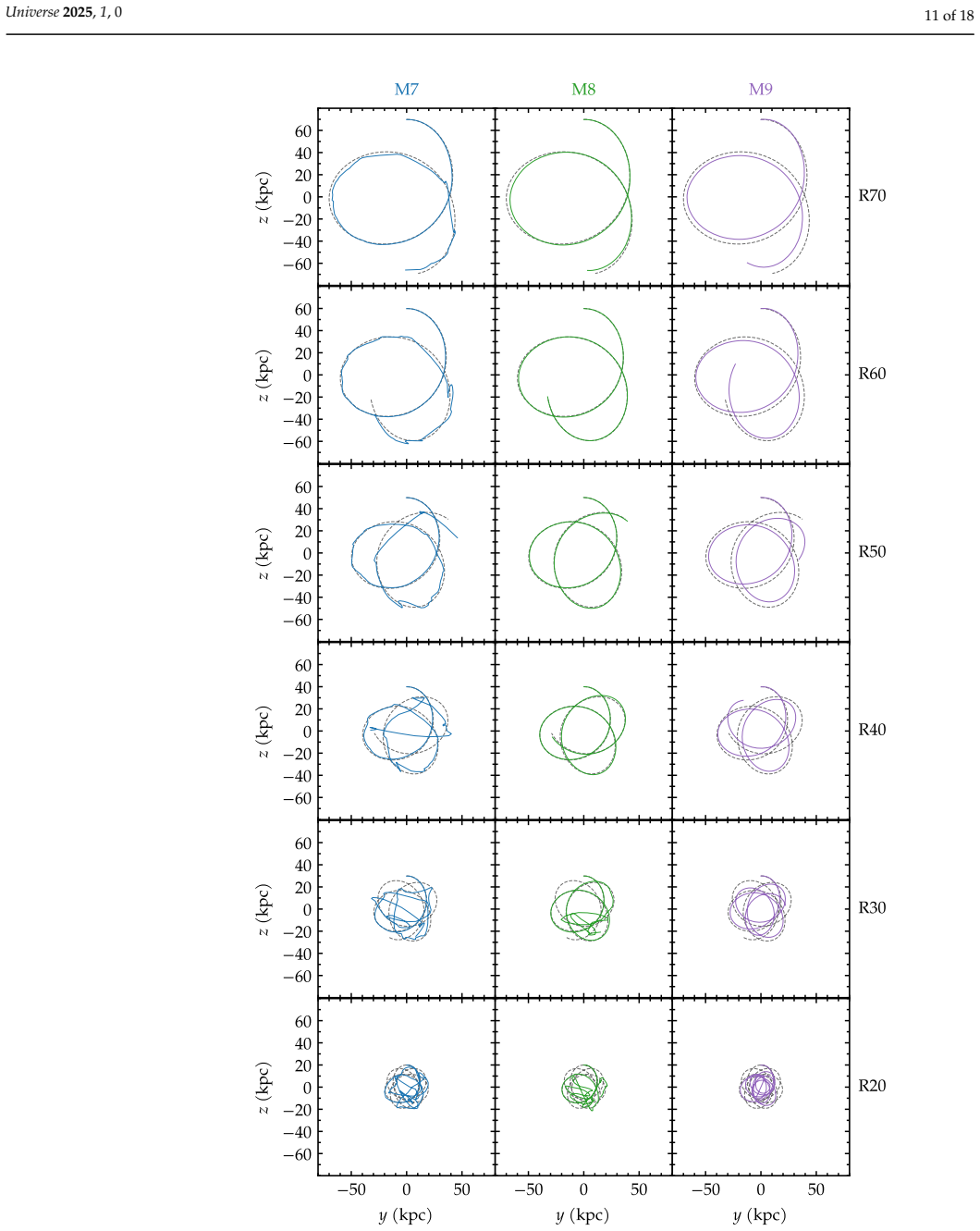
The comparison rests on two simulation setups that start from the same galaxy mass profile: a fixed analytic potential (Hernquist halo and bulge, an exponential disk represented by three Miyamoto–Nagai terms) in which the satellite is a point mass, and a live N-body realization of the same components in which the satellite is a Plummer sphere of mass $10^7$, $10^8$ or $10^9\,M_\odot$. The quantitative engine is a normalized cross-correlation (NCC) of the satellite's galactocentric-radius time series, computed between the analytic and N-body orbits; repeatedly truncating the series at earlier times gives, for each model, a cutoff $t_{\rm cut}$ at which NCC equals 0.95, defining the time span over which the orbits are considered to agree. Within those spans, the paper measures the mean relative error $|R_N - R_{\rm ana}|/R_0$ to state its accuracy limits.
What would settle it
Re-run the error analysis for all 36 models using NCC thresholds of 0.90 and 0.98 instead of 0.95; if the resulting mean errors for the $10^8\,M_\odot$ satellites fall outside the 1–5% band in either case, the advertised accuracy is an artifact of the threshold choice rather than a robust property of the orbits.
Extended reading notes
Core claim
For a host galaxy built from a Hernquist dark halo, a Hernquist bulge, and an exponential disk approximated by Miyamoto–Nagai potentials, satellite orbits computed in a static analytic potential reproduce self-consistent N-body orbits to within 5% (radius error) for satellites up to $10^8\,M_\odot$, provided the orbit is circular or moderately eccentric and the comparison is restricted to times before a normalized cross-correlation of the radial curves drops below 0.95. The most massive satellite tested, $10^9\,M_\odot$, yields 5–9% errors and, for orbits with initial radius below 30 kpc (and even at 50 kpc when eccentric), the match breaks down after roughly 1–2 Gyr. Without the time cuts, the worst mean errors reach 17% (circular) and 23% (eccentric) for the $10^9\,M_\odot$ satellite at 20 kpc.
Load-bearing premise
The headline 5% and 9% accuracy figures are computed only over time intervals ending before an arbitrary, post-hoc normalized cross-correlation threshold of 0.95; if the full 3 Gyr are included, the worst errors grow to 17–23%, so the perceived accuracy depends on choosing which time span counts.
Editorial extensions
If this is right
- For satellites up to $10^8\,M_\odot$ on circular or moderately eccentric orbits beyond 30 kpc, fast analytic-potential calculations are accurate to about 5% within the reliable window, so cheap orbital surveys and tidal-stream models built on static potentials are justified in that regime.
- A $10^9\,M_\odot$ satellite is a clear boundary: expect 5–9% errors and a reliability window of only about 2 Gyr even at 50 kpc when the orbit is eccentric, after which full N-body simulations are preferable.
- Below 30 kpc, analytic orbits of any tested mass cannot be trusted beyond about 1–2 Gyr; the paper's own uncut errors reach 17% (circular) and 23% (eccentric).
- The NCC=0.95 cutoff provides a practical criterion for deciding how long a static-potential integration remains faithful, roughly three orbital periods for the models studied.
- Tidal disruption and stream morphology should not be extrapolated from these runs: the $10^7\,M_\odot$ satellite is fully disrupted in the simulations, and the authors caution that stream conclusions depend on the artificial fixed Plummer scale length.
Reading between the lines
- The NCC=0.95 cutoff is a similarity threshold, not a physical disruption time; tying $t_{\rm cut}$ to an event like core dissolution or a fixed radial-deviation fraction would give the accuracy numbers a physical meaning they currently lack.
- The fixed Plummer radius (0.5 kpc) makes the $10^7\,M_\odot$ satellite artificially diffuse and the $10^9\,M_\odot$ one artificially concentrated; with mass-dependent sizes from dwarf scaling relations, the disruption hierarchy and reliability windows would likely shift.
- Only one eccentricity ($e \approx 0.3$) is tested; for near-radial orbits that plunge through the disk, the static potential is expected to fail much sooner, so the 5% rule should not be extrapolated to high-eccentricity orbits.
- Because the paper's errors are quoted for specific initial radii, a practical extension is to interpolate the reliability window across mass and radius to produce a trust-region map that stream-fitting pipelines could use to reject unreliable orbital segments.
Editorial analysis
A structured set of objections, weighed in public.
Referee Report
Summary. The paper compares the orbits of satellites of mass 10^7, 10^8, and 10^9 M_sun around a Milky Way-like host, computed with the analytic-potential package Gala and the N-body code Gadget-4. The setup uses polar orbits with six initial radii from 20 to 70 kpc, in both circular and moderately eccentric (initial eccentricity ~0.3) versions. The comparison metric is the mean relative difference in galactocentric radius, |R_N - R_ana|/R0, with a normalized cross-correlation (NCC) procedure used to define a 'good match' time interval t < t_cut. The headline result is that, after applying these time cuts, orbits of satellites up to 10^8 M_sun can be computed to within 5% error, while 10^9 M_sun satellites show errors of 5-9%, with reduced reliability for initial radii below 30 kpc beyond 1-2 Gyr.
Significance. The question addressed is practically important: many studies of tidal streams and satellite orbits rely on static analytic potentials, and quantitative guidance on when such potentials fail would be valuable. The paper has clear strengths: two independent implementations (Gala and Gadget-4) are compared; the parameter grid is systematic; the authors are transparent about limitations, including the fixed Plummer scale length and the explicit caveat that the summary statistics hold only when time cuts are applied. However, the headline accuracy claim is currently supported only for the radial coordinate, not for the full orbit, and the time cuts are defined by an arbitrary NCC threshold. These two issues are load-bearing for the central claim, so the manuscript needs the analysis reframed or supplemented before publication.
major comments (3)
- [§3.1, Figs. 4, 9-11] The central claim that 'orbits of satellites up to 10^8 M_sun can be reliably computed with analytic potentials to within 5% error' is supported only for the galactocentric radius, not for the full orbit. The metric |R_N - R_ana|/R0 is a radial-only measure. For the circular models, R(t) is constant for both the analytic and N-body solutions, so two trajectories on the same circle with completely different azimuthal phases produce essentially zero relative radial error. The paper itself acknowledges that phase differences matter for eccentric orbits (§3.2), but no full 3D position, angular, or phase-space error metric is reported for any model. The abstract should either be reworded to state that the 5% claim refers to galactocentric distance, or the orbital comparison should be supplemented with a 3D metric, for example the normalized instantaneous separation between the analytic and N-body positions.
- [§3.2, Eq. (1), Figs. 8-11] The headline 5% and 9% error figures are computed only within time intervals t < t_cut that are defined by the arbitrary requirement NCC >= 0.95. The same NCC measure is used both to decide which times are 'reliable' and to justify the reported errors, making the accuracy numbers partly a consequence of the chosen threshold. Without these cuts, the mean relative errors reach 17% for the circular M9R20 model and 23% for the eccentric M9R20 model (Fig. 10). The paper is transparent about this in Section 4 ('these summary statistics hold only if the time cuts are applied'), but the abstract presents the numbers as unconditional. The authors should either (i) state the unconditional error values alongside the conditional ones in the abstract, or (ii) motivate the NCC = 0.95 threshold using an independent, physically grounded criterion, such as a maximum permitted mass-loss fraction, survival of a bound core, or a maximum allowed radial offset.
- [§2.2, §4, Figs. 1 and 5] The fixed Plummer scale length a = 0.5 kpc for all three satellite masses is a notable limitation for the stream-disruption analysis, as the authors acknowledge. Because the low-mass satellite is less centrally concentrated, it is more easily disrupted, and the systematic differences in stream morphology among the M7, M8, and M9 models are partly an artifact of this choice. This also feeds into the orbital comparison for the M7 cases, where the authors state that the satellite center becomes ill-defined. The paper's caveat about stream-formation conclusions is appropriate, but the orbital comparison would be strengthened by a quantitative assessment of how much of the low-mass orbital error is attributable to the difficulty of defining the satellite center rather than to genuine dynamical divergence.
minor comments (4)
- [§2.1] There are several typographical errors: 'valocities' for 'velocities' in the sentence introducing Table 1, 'trully' for 'truly', and 'correponding' for 'corresponding' elsewhere in the text.
- [§3.1, §3.2, Figs. 4, 9] Figure 9 reports mean relative errors with open symbols for the t < t_cut restricted data, but those open-symbol values are shown without uncertainty estimates, unlike the full-symbol values in Figures 4 and 9. Adding error bars or scatter ranges for the restricted means would improve the interpretability of the comparison.
- [§3.2, text near Eq. (1)] The phrase 'a gives time' appears to be a typo; it should likely read 'at a given time.'
- [References [33,34]] The text cites 'Gadget-4 code [33,34]' but reference [33] is the GADGET-2 paper, not a paper on GADGET-4. Consider citing the original GADGET-2 paper separately when the code architecture is discussed and reserving [34] for the GADGET-4 code.
Circularity Check
No significant circularity: the benchmark compares two independent integrators and reports conditional errors; the time-cut qualifier is disclosed, not a fitted prediction.
full rationale
The paper's central claim is an empirical comparison, not a derivation. The analytic orbits are computed by integrating a fixed potential with Gala (Section 2.1), and the N-body orbits are produced by Gadget-4 from independently realized particle initial conditions (Section 2.2). No parameter is fitted to the N-body output and then renamed as a prediction. The only protocol choice that could look circular is the t<t_cut restriction: Section 3.2 defines t_cut as the time at which the normalized cross-correlation of the radial curves reaches an arbitrary threshold of 0.95, and Figs. 9-11 then report mean radial errors computed only within that interval. However, the NCC threshold does not, by construction, set the mean relative error to 5% or 9%; it merely selects the interval over which the comparison is quoted. The paper is explicit about this conditionality: 'It should be emphasized that these summary statistics hold only if the time cuts are applied.' That is a disclosed limitation, not a hidden reduction of the output to the input. Separately, the metric is the galactocentric radius only, so the phrase 'orbits' may overstate the scope of the 5%/9% numbers; that is a correctness or validity concern, not circularity. There are no load-bearing self-citations, no imported uniqueness theorems, and no renamed known result. The comparison is self-contained and externally falsifiable.
Assumptions & free parameters
free parameters (3)
- NCC threshold =
0.95
- Plummer scale length a =
0.5 kpc
- Eccentric velocity factor =
0.7
assumptions (5)
- domain assumption Hernquist profiles for halo and bulge plus Miyamoto-Nagai disks provide an adequate Milky Way-like gravitational model
- domain assumption The chosen orbit family (polar, e ~ 0.3) is representative of the regimes where the error calibration is claimed
- ad hoc to paper NCC >= 0.95 is a valid criterion for defining the reliable time interval
- domain assumption A single Plummer sphere with fixed scale length represents the satellite galaxy
- standard math Newtonian gravity and collisionless N-body dynamics apply at the scales considered
Cite this review
Pith. "Pith review of Accuracy of analytic potentials for orbits of satellites around a Milky Way-like galaxy: comparison with $N$-body simulations." pith.science (2026). https://pith.science/paper/BYY2CKLY
@misc{pith2026250613813,
  author       = {Pith},
  title        = {Pith review of: Accuracy of analytic potentials for orbits of satellites around a Milky Way-like galaxy: comparison with $N$-body simulations},
  year         = {2026},
  howpublished = {\url{https://pith.science/paper/BYY2CKLY}},
  note         = {Machine review of arXiv:2506.13813}
}
abstract
To study the orbits of satellites, a galaxy could be modelled either by means of a static gravitational potential, or by live $N$-body particles. Analytic potentials allow for fast calculations, but are idealized and non-responsive. On the other hand, $N$-body simulations are more realistic, but demand higher computational cost. Our goal is to characterize the regimes in which analytic potentials provide a sufficient approximation, and those where $N$-bodies are necessary. We perform two sets of simulations using both Gala and Gadget, in order to closely compare the orbital evolution of satellites around a Milky Way-like galaxy. Focusing on the periods when the satellite has not yet been severely disrupted by tidal forces, we find that the orbits of satellites up to $10^{8} {\rm M_{\odot}}$ can be reliably computed with analytic potentials to within 5% error, if they are circular or moderately eccentric. If the satellite is as massive as $10^{9} {\rm M_{\odot}}$, errors of 9% are to be expected. However, if the orbital radius is smaller than 30 kpc, the results may not be relied upon with the same accuracy beyond 1--2 Gyr.
Figures


Figures from the paper (8 more)




Reference graph
Works this paper leans on
-
[1]
Gaia Collaboration.; Prusti, T.; de Bruijne, J.H.J.; Brown, A.G.A.; Vallenari, A.; Babusiaux, C.; Bailer-Jones, C.A.L.; Bastian, U.; Biermann, M.; Evans, D.W.; et al. The Gaia mission.Astron. Astrophys.2016,595, A1, [arXiv:astro-ph.IM/1609.04153]. https://doi.org/10.1051/0004-6361/201629272
arXiv 2016
-
[2]
Gaia Collaboration.; Brown, A.G.A.; Vallenari, A.; Prusti, T.; de Bruijne, J.H.J.; Mignard, F.; Drimmel, R.; Babusiaux, C.; Bailer- Jones, C.A.L.; Bastian, U.; et al. Gaia Data Release 1. Summary of the astrometric, photometric, and survey properties.Astron. Astrophys.2016,595, A2, [arXiv:astro-ph.IM/1609.04172]. https://doi.org/10.1051/0004-6361/201629512
arXiv 2016
-
[3]
Gaia Collaboration.; Brown, A.G.A.; Vallenari, A.; Prusti, T.; de Bruijne, J.H.J.; Babusiaux, C.; Bailer-Jones, C.A.L.; Biermann, M.; Evans, D.W.; Eyer, L.; et al. Gaia Data Release 2. Summary of the contents and survey properties.Astron. Astrophys.2018,616, A1, [arXiv:astro-ph.GA/1804.09365]. https://doi.org/10.1051/0004-6361/201833051
arXiv 2018
-
[4]
Gaia Collaboration.; Brown, A.G.A.; Vallenari, A.; Prusti, T.; de Bruijne, J.H.J.; Babusiaux, C.; Biermann, M.; Creevey, O.L.; Evans, D.W.; Eyer, L.; et al. Gaia Early Data Release 3. Summary of the contents and survey properties.Astron. Astrophys.2021,649, A1, [arXiv:astro-ph.GA/2012.01533]. https://doi.org/10.1051/0004-6361/202039657
arXiv 2021
-
[5]
Gaia Collaboration.; Vallenari, A.; Brown, A.G.A.; Prusti, T.; de Bruijne, J.H.J.; Arenou, F.; Babusiaux, C.; Biermann, M.; Creevey, O.L.; Ducourant, C.; et al. Gaia Data Release 3. Summary of the content and survey properties.Astron. Astrophys.2023,674, A1, [arXiv:astro-ph.GA/2208.00211]. https://doi.org/10.1051/0004-6361/202243940
arXiv 2023
-
[6]
A dwarf satellite galaxy in Sagittarius.Nature1994,370, 194–196
Ibata, R.A.; Gilmore, G.; Irwin, M.J. A dwarf satellite galaxy in Sagittarius.Nature1994,370, 194–196. https://doi.org/10.1038/ 370194a0
-
[7]
Sagittarius: The Nearest Dwarf Galaxy
Ibata, R.A.; Gilmore, G.; Irwin, M.J. Sagittarius: the nearest dwarf galaxy.Mon. Not. R. Astron. Soc.1995,277, 781–800, [arXiv:astro-ph/astro-ph/9506071]. https://doi.org/10.1093/mnras/277.3.781
work page Pith review arXiv 1995
-
[8]
Odenkirchen, M.; Grebel, E.K.; Rockosi, C.M.; Dehnen, W.; Ibata, R.; Rix, H.W.; Stolte, A.; Wolf, C.; Anderson, John E., J.; Bahcall, N.A.; et al. Detection of Massive Tidal Tails around the Globular Cluster Palomar 5 with Sloan Digital Sky Survey Commissioning Data.Astrophys. J. Lett.2001,548, L165–L169, [arXiv:astro-ph/astro-ph/0012311]. https://doi.org...
arXiv 2001
Show all 39 references
-
[9]
A Matched-Filter Analysis of the Tidal Tails of the Globular Cluster Palomar 5.The Astronomical Journal2002, 124, 349–363
Rockosi, C.M.; Odenkirchen, M.; Grebel, E.K.; Dehnen, W.; Cudworth, K.M.; Gunn, J.E.; York, D.G.; Brinkmann, J.; Hennessy, G.S.; Ivezi´ c, Ž. A Matched-Filter Analysis of the Tidal Tails of the Globular Cluster Palomar 5.The Astronomical Journal2002, 124, 349–363. https://doi....
-
[10]
Streams, Substructures, and the Early History of the Milky Way.Annu
Helmi, A. Streams, Substructures, and the Early History of the Milky Way.Annu. Rev. Astron. Astrophys.2020,58, 205–256, [arXiv:astro-ph.GA/2002.04340]. https://doi.org/10.1146/annurev-astro-032620-021917
2020 arXiv
-
[11]
galstreams: A library of Milky Way stellar stream footprints and tracks.Mon
Mateu, C. galstreams: A library of Milky Way stellar stream footprints and tracks.Mon. Not. R. Astron. Soc.2023,520, 5225–5258, [arXiv:astro-ph.GA/2204.10326]. https://doi.org/10.1093/mnras/stad321
2023 arXiv
-
[12]
Charting the Galactic Acceleration Field
Ibata, R.; Malhan, K.; Tenachi, W.; Ardern-Arentsen, A.; Bellazzini, M.; Bianchini, P .; Bonifacio, P .; Caffau, E.; Diakogiannis, F.; Errani, R.; et al. Charting the Galactic Acceleration Field. II. A Global Mass Model of the Milky Way from the STREAMFINDER Atlas of Stellar S...
2024 arXiv
-
[13]
Stellar streams in the Gaia era.New Astron.2025,100, 101713, [arXiv:astro-ph.GA/2405.19410]
Bonaca, A.; Price-Whelan, A.M. Stellar streams in the Gaia era.New Astron.2025,100, 101713, [arXiv:astro-ph.GA/2405.19410]. https://doi.org/10.1016/j.newar.2024.101713
2025 arXiv
-
[14]
On N-body simulations of globular cluster streams.Mon
Banik, N.; Bovy, J. On N-body simulations of globular cluster streams.Mon. Not. R. Astron. Soc.2021,504, 648–653, [arXiv:astro-ph.GA/2101.12201]. https://doi.org/10.1093/mnras/stab886
2021 arXiv
-
[15]
Milky Way Mass and Potential Recovery Using Tidal Streams in a Realistic Halo.Astrophys
Bonaca, A.; Geha, M.; Küpper, A.H.W.; Diemand, J.; Johnston, K.V .; Hogg, D.W. Milky Way Mass and Potential Recovery Using Tidal Streams in a Realistic Halo.Astrophys. J.2014,795, 94, [arXiv:astro-ph.GA/1406.6063]. https://doi.org/10.1088/0004-637X/ 795/1/94
2014 arXiv
-
[16]
galpy: A python Library for Galactic Dynamics.Astrophys
Bovy, J. galpy: A python Library for Galactic Dynamics.Astrophys. J. Suppl. Ser.2015,216, 29, [arXiv:astro-ph.GA/1412.3451]. https://doi.org/10.1088/0067-0049/216/2/29. Universe2025,1, 0 18 of 18
2015 arXiv
-
[17]
The mass distribution and gravitational potential of the Milky Way.Mon
McMillan, P .J. The mass distribution and gravitational potential of the Milky Way.Mon. Not. R. Astron. Soc.2017,465, 76–94, [arXiv:astro-ph.GA/1608.00971]. https://doi.org/10.1093/mnras/stw2759
2017 arXiv
-
[18]
Gala: A Python package for galactic dynamics.The Journal of Open Source Software2017,2, 388
Price-Whelan, A.M. Gala: A Python package for galactic dynamics.The Journal of Open Source Software2017,2, 388. https: //doi.org/10.21105/joss.00388
-
[19]
Uncertainties associated with the backward integration of dwarf satellites using simple parametric potentials
D’Souza, R.; Bell, E.F. Uncertainties associated with the backward integration of dwarf satellites using simple parametric potentials. Mon. Not. R. Astron. Soc.2022,512, 739–760, [arXiv:astro-ph.GA/2202.05707]. https://doi.org/10.1093/mnras/stac404
2022 arXiv
-
[20]
Modelling the orbital histories of satellites of Milky Way-mass galaxies: testing static host potentials against cosmological simulations.Mon
Santistevan, I.B.; Wetzel, A.; Tollerud, E.; Sanderson, R.E.; Moreno, J.; Patel, E. Modelling the orbital histories of satellites of Milky Way-mass galaxies: testing static host potentials against cosmological simulations.Mon. Not. R. Astron. Soc.2024,527, 8841–8864, [arXiv:as...
2024 arXiv
-
[21]
The last breath of the Sagittarius dSph.Mon
Vasiliev, E.; Belokurov, V . The last breath of the Sagittarius dSph.Mon. Not. R. Astron. Soc.2020,497, 4162–4182, [arXiv:astro- ph.GA/2006.02929]. https://doi.org/10.1093/mnras/staa2114
2020 arXiv
-
[22]
Tango for three: Sagittarius, LMC, and the Milky Way.Mon
Vasiliev, E.; Belokurov, V .; Erkal, D. Tango for three: Sagittarius, LMC, and the Milky Way.Mon. Not. R. Astron. Soc.2021, 501, 2279–2304, [arXiv:astro-ph.GA/2009.10726]. https://doi.org/10.1093/mnras/staa3673
2021 arXiv
-
[23]
And Yet it Moves: The Dangers of Artificially Fixing the Milky Way Center of Mass in the Presence of a Massive Large Magellanic Cloud.Astrophys
Gómez, F.A.; Besla, G.; Carpintero, D.D.; Villalobos, Á.; O’Shea, B.W.; Bell, E.F. And Yet it Moves: The Dangers of Artificially Fixing the Milky Way Center of Mass in the Presence of a Massive Large Magellanic Cloud.Astrophys. J.2015,802, 128, [arXiv:astro-ph.GA/1408.4128]. h...
2015 arXiv
-
[24]
Reconstructing the Last Major Merger of the Milky Way with the H3 Survey.Astrophys
Naidu, R.P .; Conroy, C.; Bonaca, A.; Zaritsky, D.; Weinberger, R.; Ting, Y.S.; Caldwell, N.; Tacchella, S.; Han, J.J.; Speagle, J.S.; et al. Reconstructing the Last Major Merger of the Milky Way with the H3 Survey.Astrophys. J.2021,923, 92, [arXiv:astro- ph.GA/2103.03251]. ht...
2021 arXiv
-
[25]
Gaps and length asymmetry in the stellar stream Palomar 5 as effects of Galactic bar rotation.Nature Astronomy2017,1, 633–639, [arXiv:astro-ph.GA/1703.04627]
Pearson, S.; Price-Whelan, A.M.; Johnston, K.V . Gaps and length asymmetry in the stellar stream Palomar 5 as effects of Galactic bar rotation.Nature Astronomy2017,1, 633–639, [arXiv:astro-ph.GA/1703.04627]. https://doi.org/10.1038/s41550-017-0220-3
-
[26]
On the Stability of Tidal Streams in Action Space.Astrophys
Arora, A.; Sanderson, R.E.; Panithanpaisal, N.; Cunningham, E.C.; Wetzel, A.; Garavito-Camargo, N. On the Stability of Tidal Streams in Action Space.Astrophys. J.2022,939, 2, [arXiv:astro-ph.GA/2207.13481]. https://doi.org/10.3847/1538-4357/ac93fb
2022 arXiv
-
[27]
Generation of mock tidal streams.Mon
Fardal, M.A.; Huang, S.; Weinberg, M.D. Generation of mock tidal streams.Mon. Not. R. Astron. Soc.2015,452, 301–319, [arXiv:astro-ph.GA/1410.1861]. https://doi.org/10.1093/mnras/stv1198
2015 arXiv
-
[28]
An analytical model for spherical galaxies and bulges.Astrophys
Hernquist, L. An analytical model for spherical galaxies and bulges.Astrophys. J.1990,356, 359–364. https://doi.org/10.1086/16 8845
1990 doi
-
[29]
Three-dimensional models for the distribution of mass in galaxies.Publ
Miyamoto, M.; Nagai, R. Three-dimensional models for the distribution of mass in galaxies.Publ. Astron. Soc. Jpn.1975, 27, 533–543
1975
-
[30]
Simple and accurate modelling of the gravitational potential produced by thick and thin exponential discs.Mon
Smith, R.; Flynn, C.; Candlish, G.N.; Fellhauer, M.; Gibson, B.K. Simple and accurate modelling of the gravitational potential produced by thick and thin exponential discs.Mon. Not. R. Astron. Soc.2015,448, 2934–2940, [arXiv:astro-ph.GA/1502.00627]. https://doi.org/10.1093/mnr...
2015 arXiv
-
[31]
The fate of the gaseous discs of galaxies that fall into clusters.Mon
Ruggiero, R.; Lima Neto, G.B. The fate of the gaseous discs of galaxies that fall into clusters.Mon. Not. R. Astron. Soc.2017, 468, 4107–4115, [1703.08550]. https://doi.org/10.1093/mnras/stx744
2017 arXiv
-
[32]
On the problem of distribution in globular star clusters.Mon
Plummer, H.C. On the problem of distribution in globular star clusters.Mon. Not. R. Astron. Soc.1911,71, 460–470. https://doi.org/10.1093/mnras/71.5.460
1911 doi
-
[33]
The cosmological simulation code GADGET-2.Mon
Springel, V . The cosmological simulation code GADGET-2.Mon. Not. R. Astron. Soc.2005,364, 1105–1134, [arXiv:astro- ph/0505010]. https://doi.org/10.1111/j.1365-2966.2005.09655.x
2005
-
[34]
Simulating cosmic structure formation with the GADGET-4 code.Mon
Springel, V .; Pakmor, R.; Zier, O.; Reinecke, M. Simulating cosmic structure formation with the GADGET-4 code.Mon. Not. R. Astron. Soc.2021,506, 2871–2949, [arXiv:astro-ph.IM/2010.03567]. https://doi.org/10.1093/mnras/stab1855
2021 arXiv
-
[35]
The Accuracy of Cross-Correlation Estimates of Quasar Emission-Line Region Sizes.Astrophys
Gaskell, C.M.; Peterson, B.M. The Accuracy of Cross-Correlation Estimates of Quasar Emission-Line Region Sizes.Astrophys. J. Suppl. Ser.1987,65, 1. https://doi.org/10.1086/191216
1987 doi
-
[36]
Cross-correlation and maximum-likelihood analysis: a new approach to combining cross-correlation functions.Mon
Zucker, S. Cross-correlation and maximum-likelihood analysis: a new approach to combining cross-correlation functions.Mon. Not. R. Astron. Soc.2003,342, 1291–1298, [arXiv:astro-ph/astro-ph/0303426]. https://doi.org/10.1046/j.1365-8711.2003.06633.x
2003 arXiv
-
[37]
The size distribution of galaxies in the Sloan Digital Sky Survey.Mon
Shen, S.; Mo, H.J.; White, S.D.M.; Blanton, M.R.; Kauffmann, G.; Voges, W.; Brinkmann, J.; Csabai, I. The size distribution of galaxies in the Sloan Digital Sky Survey.Mon. Not. R. Astron. Soc.2003,343, 978–994, [arXiv:astro-ph/astro-ph/0301527]. https://doi.org/10.1046/j.1365...
2003 arXiv
-
[38]
Galaxy And Mass Assembly (GAMA): mass-size relations of z < 0.1 galaxies subdivided by Sérsic index, colour and morphology.Mon
Lange, R.; Driver, S.P .; Robotham, A.S.G.; Kelvin, L.S.; Graham, A.W.; Alpaslan, M.; Andrews, S.K.; Baldry, I.K.; Bamford, S.; Bland-Hawthorn, J.; et al. Galaxy And Mass Assembly (GAMA): mass-size relations of z < 0.1 galaxies subdivided by Sérsic index, colour and morphology...
2015 arXiv
-
[39]
The stellar mass - physical effective radius relation for dwarf galaxies in low-density environments.Mon
Prole, D.J. The stellar mass - physical effective radius relation for dwarf galaxies in low-density environments.Mon. Not. R. Astron. Soc.2021,506, L59–L63, [arXiv:astro-ph.GA/2106.14924]. https://doi.org/10.1093/mnrasl/slab073. Disclaimer/Publisher’s Note:The statements, opin...
2021 arXiv
Reviewed August 7, 2026 · model on record in the stance chip above.
Discussion (0). Sign in to comment.