Extracting transient Koopman modes from short-term weather simulations with sparsity-promoting dynamic mode decomposition
Pith reviewed 2026-05-19 10:02 UTC · model grok-4.3
The pith
Sparsity-promoting dynamic mode decomposition extracts sparse transient Koopman modes that track the growth and decay of bubble-like patterns in short-term weather simulations.
A machine-rendered reading of the paper's core claim, the machinery that carries it, and where it could break.
Core claim
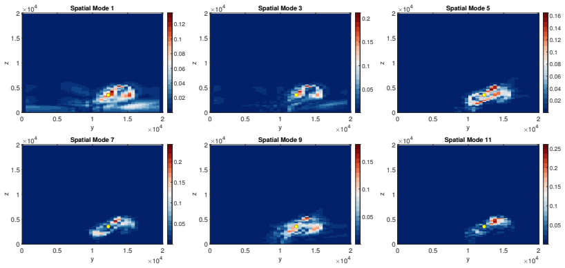
By using sparsity-promoting dynamic mode decomposition on short-term weather simulation data with velocity and vorticity magnitude as observables, the work obtains a sparse collection of dominant Koopman modes. These modes represent the transient evolution of warm bubble-like convective patterns. Adjusting the sparsity weight trades off between reconstruction fidelity and the number of retained modes, resulting in a reduced-order model that acts as a surrogate for the full weather system in diagnostic and forecasting contexts.
What carries the argument
Sparsity-promoting dynamic mode decomposition that promotes sparse amplitudes in the modal expansion to select the dominant transient Koopman modes from the data.
If this is right
- The transient convective structures can be represented with significantly fewer degrees of freedom than the original high-dimensional simulation.
- Tuning the sparsity weight provides control over the complexity of the reduced model while maintaining reconstruction quality.
- The extracted modes enable the creation of low-dimensional surrogates suitable for repeated diagnostic evaluations.
- Forecasting tasks can potentially leverage these modes for faster computation of short-term evolution.
Where Pith is reading between the lines
- If these modes prove robust across varying simulation conditions, they could serve as building blocks for hybrid physics-informed forecasting systems.
- Applying the same extraction process to other observable quantities might uncover additional transient features not visible in velocity or vorticity alone.
- This dimensionality reduction technique could be tested on real observational data rather than just simulations to assess practical utility.
Load-bearing premise
Short-term weather dynamics are sufficiently linear in the chosen observables of velocity and vorticity magnitudes for the sparsity-promoting decomposition to isolate the relevant transient structures.
What would settle it
If the reconstructed fields from the sparse modes do not accurately reproduce the bubble-like patterns observed in held-out weather simulations, the effectiveness of the extracted modes for representing the dynamics would be called into question.
Figures


read the original abstract
Convective features, represented here as warm bubble-like patterns, reveal essential high-level information about how short-term weather dynamics evolve within a high-dimensional state space. In this paper, we introduce a data-driven framework that uncovers transient dynamics captured by Koopman modes responsible for these structures and traces their emergence, growth, and decay. Our approach applies the sparsity-promoting dynamic mode decomposition to weather simulations, yielding a few number of selected modes whose sparse amplitudes highlight dominant transient structures. By tuning the sparsity weight, we balance reconstruction accuracy and model complexity. We illustrate the methodology on weather simulations, using the magnitude of velocity and vorticity fields as distinct observable datasets. The resulting sparse dominant Koopman modes capture the transient evolution of bubble-like pattern and can reduce the dimensionality of weather system model, offering an efficient surrogate for diagnostic and forecasting tasks.
Editorial analysis
A structured set of objections, weighed in public.
Referee Report
Summary. The paper introduces a data-driven framework applying sparsity-promoting dynamic mode decomposition (DMD) to short-term weather simulations. Using magnitudes of velocity and vorticity fields as observables, it tunes a sparsity weight to select a small number of Koopman modes claimed to capture the emergence, growth, and decay of bubble-like convective patterns, thereby reducing dimensionality for surrogate diagnostic and forecasting tasks.
Significance. If the linear Koopman approximation holds and the extracted modes are validated, the approach could provide an efficient reduced-order representation of transient convective structures in high-dimensional weather data. The application of sparsity-promoting DMD to this setting has potential utility, but the manuscript offers no quantitative metrics to confirm that the selected modes faithfully represent the underlying nonlinear dynamics rather than merely reproducing snapshot patterns.
major comments (2)
- [Abstract] Abstract: the central claim that 'the resulting sparse dominant Koopman modes capture the transient evolution of bubble-like pattern' is unsupported by any reported reconstruction errors, prediction accuracy on held-out data, baseline comparisons (e.g., to standard DMD or POD), or error bars; without these the support for faithful representation of transient convective structures is weak.
- [Methodology/Results] Methodology/Results: mode selection and dominance are controlled by the manually tuned sparsity weight chosen to balance accuracy and complexity; this hyperparameter directly determines which modes are retained, creating a circular dependence that undermines the claim of purely data-driven extraction of transient dynamics.
minor comments (2)
- [Methodology] Clarify the precise definition of the observable functions (velocity and vorticity magnitudes) and the lifting to the Koopman space; the linear operator assumption for strongly nonlinear advection and buoyancy effects requires explicit justification.
- [Results] Add sensitivity analysis or cross-validation for the sparsity weight choice and report the number of retained modes and their amplitudes for the presented simulations.
Simulated Author's Rebuttal
We thank the referee for the constructive comments on our manuscript. We address each major comment below and indicate revisions where appropriate to strengthen the quantitative support and clarify the methodology.
read point-by-point responses
-
Referee: [Abstract] Abstract: the central claim that 'the resulting sparse dominant Koopman modes capture the transient evolution of bubble-like pattern' is unsupported by any reported reconstruction errors, prediction accuracy on held-out data, baseline comparisons (e.g., to standard DMD or POD), or error bars; without these the support for faithful representation of transient convective structures is weak.
Authors: We acknowledge that the abstract statement would benefit from explicit quantitative backing. The current manuscript demonstrates the modes primarily through visualizations of their spatial structures and temporal coefficients matching the emergence and decay of convective patterns. In the revision we will add a dedicated quantitative validation subsection reporting reconstruction errors on the training snapshots, comparisons against standard DMD and POD baselines, and sensitivity analysis with error bars. revision: yes
-
Referee: [Methodology/Results] Methodology/Results: mode selection and dominance are controlled by the manually tuned sparsity weight chosen to balance accuracy and complexity; this hyperparameter directly determines which modes are retained, creating a circular dependence that undermines the claim of purely data-driven extraction of transient dynamics.
Authors: The sparsity weight is a regularization parameter whose role is explicitly described in the sparsity-promoting DMD formulation we employ. Its value is selected to yield a small number of modes whose amplitudes highlight the dominant transient convective features observed in the data; this is standard practice for the method and does not create circularity—the modes themselves are computed directly from the snapshot data via the DMD operator. We will expand the methodology section to include a brief sensitivity study showing how the retained modes vary with the weight and to clarify that the data-driven extraction occurs prior to the final sparsity thresholding. revision: partial
Circularity Check
Sparsity weight tuning directly shapes which Koopman modes are retained as dominant
specific steps
-
fitted input called prediction
[Abstract]
"By tuning the sparsity weight, we balance reconstruction accuracy and model complexity. ... The resulting sparse dominant Koopman modes capture the transient evolution of bubble-like pattern and can reduce the dimensionality of weather system model"
The sparsity weight is adjusted to achieve the desired balance; the modes labeled 'resulting' and 'dominant' are then asserted to capture the transient evolution. Because mode retention and dominance are controlled by this fitted hyperparameter, the claim that the sparse modes faithfully represent the convective structures is statistically forced by the tuning step rather than independently verified.
full rationale
The paper's central claim that the extracted modes capture transient bubble-like evolution rests on a manually tuned sparsity weight that balances reconstruction accuracy against model complexity. This hyperparameter choice determines mode selection and dominance, so the reported 'resulting sparse dominant Koopman modes' are shaped by the fit rather than emerging independently from the data-driven operator. The underlying DMD is data-driven, but the load-bearing step of declaring the selected modes faithful to the transient structures reduces to this tuned input.
Axiom & Free-Parameter Ledger
free parameters (1)
- sparsity weight
axioms (1)
- domain assumption Short-term weather dynamics admit a useful finite-dimensional linear approximation in the Koopman sense when projected onto velocity and vorticity magnitude observables.
Lean theorems connected to this paper
-
IndisputableMonolith/Cost/FunctionalEquation.leanwashburn_uniqueness_aczel unclear?
unclearRelation between the paper passage and the cited Recognition theorem.
Our approach incorporates the sparsity-promoting dynamic mode decomposition into the framework of Koopman mode decomposition, yielding a few number of selected modes whose sparse amplitudes highlight dominant transient structures. By tuning the sparsity weight, we balance reconstruction accuracy and model complexity.
-
IndisputableMonolith/Foundation/RealityFromDistinction.leanreality_from_one_distinction unclear?
unclearRelation between the paper passage and the cited Recognition theorem.
the resulting sparse dominant Koopman modes capture the transient evolution of bubble-like pattern
What do these tags mean?
- matches
- The paper's claim is directly supported by a theorem in the formal canon.
- supports
- The theorem supports part of the paper's argument, but the paper may add assumptions or extra steps.
- extends
- The paper goes beyond the formal theorem; the theorem is a base layer rather than the whole result.
- uses
- The paper appears to rely on the theorem as machinery.
- contradicts
- The paper's claim conflicts with a theorem or certificate in the canon.
- unclear
- Pith found a possible connection, but the passage is too broad, indirect, or ambiguous to say the theorem truly supports the claim.
Reference graph
Works this paper leans on
-
[1]
D. L. Hartmann, Global physical climatology. Newnes, 2015, vol. 103
work page 2015
-
[2]
Pedlosky, Geophysical fluid dynamics
J. Pedlosky, Geophysical fluid dynamics . Springer Science & Business Media, 2013
work page 2013
-
[3]
S. Kotsuki, Y. Sato, and T. Miyoshi, “Data assimilation for climate research: model parameter estimation of large-scale condensation scheme,” J. Geophys. Res., vol. 125, no. 1, p. e2019JD031304, 2020
work page 2020
-
[4]
E. N. Lorenz, Empirical orthogonal functions and statistical weather prediction . Massachusetts Institute of Technology, Department of Meteorology Cambridge, 1956, vol. 1
work page 1956
-
[5]
Empirical orthogonal func- tions and related techniques in atmospheric science: A review,
A. Hannachi, I. T. Jolliffe, D. B. Stephenson et al. , “Empirical orthogonal func- tions and related techniques in atmospheric science: A review,” Int. J. Climatol. , vol. 27, no. 9, pp. 1119–1152, 2007
work page 2007
-
[6]
Spectral empirical orthogonal function analysis of weather and climate data,
O. T. Schmidt, G. Mengaldo, G. Balsamo, and N. P. Wedi, “Spectral empirical orthogonal function analysis of weather and climate data,” Mon. Weather Rev. , vol. 147, no. 8, pp. 2979–2995, 2019
work page 2019
-
[7]
D. Giannakis and A. J. Majda, “Nonlinear Laplacian spectral analysis for time series with intermittency and low-frequency variability,” Proc. Natl. Acad. Sci. , vol. 109, no. 7, pp. 2222–2227, 2012
work page 2012
-
[8]
H.-D. Chiang, Direct methods for stability analysis of electric power systems: The- oretical foundation, BCU methodologies, and applications . John Wiley & Sons, 2011
work page 2011
-
[9]
Hydrodynamic stability without eigenvalues,
L. N. Trefethen, A. E. Trefethen, S. C. Reddy, and T. A. Driscoll, “Hydrodynamic stability without eigenvalues,” Science, vol. 261, no. 5121, pp. 578–584, 1993
work page 1993
- [10]
-
[11]
A cautionary note on the interpretation of EOFs,
D. Dommenget and M. Latif, “A cautionary note on the interpretation of EOFs,” J. Clim., vol. 15, no. 2, pp. 216–225, 2002
work page 2002
-
[12]
Variability of SST through Koopman modes,
A. Navarra, J. Tribbia, S. Klus, and P. Lorenzo-S´ anchez, “Variability of SST through Koopman modes,” J. Clim., 2024
work page 2024
-
[13]
Linear inverse modeling of large-scale atmospheric flow using opti- mal mode decomposition,
F. Kwasniok, “Linear inverse modeling of large-scale atmospheric flow using opti- mal mode decomposition,” J. Atmos. Sci. , vol. 79, no. 9, pp. 2181–2204, 2022. 32
work page 2022
-
[14]
The role of sea surface salinity in ENSO forecasting in the 21st century,
H. Wang, S. Hu, C. Guan, and X. Li, “The role of sea surface salinity in ENSO forecasting in the 21st century,”NPJ Clim. Atmos. Sci., vol. 7, no. 1, p. 206, 2024
work page 2024
-
[15]
Hamiltonian systems and transformation in Hilbert space,
B. O. Koopman, “Hamiltonian systems and transformation in Hilbert space,” Proc. Natl. Acad. Sci., vol. 17, no. 5, pp. 315–318, 1931
work page 1931
-
[16]
Spectral properties of dynamical systems, model reduction and decom- positions,
I. Mezi´ c, “Spectral properties of dynamical systems, model reduction and decom- positions,” Nonlinear Dynamics, vol. 41, pp. 309–325, 2005
work page 2005
-
[17]
Spectral analysis of nonlinear flows,
C. W. Rowley, I. Mezi´ c, S. Bagheri, P. Schlatter, and D. S. Henningson, “Spectral analysis of nonlinear flows,” J. Fluid Mech. , vol. 641, pp. 115–127, 2009
work page 2009
-
[18]
Dynamic mode decomposition of numerical and experimental data,
P. J. Schmid, “Dynamic mode decomposition of numerical and experimental data,” J. Fluid Mech. , vol. 656, pp. 5–28, 2010
work page 2010
-
[19]
Analysis of fluid flows via spectral properties of the Koopman operator,
I. Mezi´ c, “Analysis of fluid flows via spectral properties of the Koopman operator,” Annu. Rev. Fluid Mech. , vol. 45, no. 1, pp. 357–378, 2013
work page 2013
-
[20]
Dy- namic mode decomposition: Theory and applications,
J. H. Tu, C. W. Rowley, D. M. Luchtenburg, S. L. Brunton, and J. N. Kutz, “Dy- namic mode decomposition: Theory and applications,” J. Comput. Dyn. , vol. 1, no. 2, pp. 391–421, 2014
work page 2014
-
[21]
Sparsity-promoting dynamic mode decomposition,
M. R. Jovanovi´ c, P. J. Schmid, and J. W. Nichols, “Sparsity-promoting dynamic mode decomposition,” Phys. Fluids, vol. 26, no. 2, 2014
work page 2014
-
[22]
A data–driven approxi- mation of the Koopman operator: Extending dynamic mode decomposition,
M. O. Williams, I. G. Kevrekidis, and C. W. Rowley, “A data–driven approxi- mation of the Koopman operator: Extending dynamic mode decomposition,” J. Nonlinear Sci., vol. 25, pp. 1307–1346, 2015
work page 2015
-
[23]
J. N. Kutz, S. L. Brunton, B. W. Brunton, and J. L. Proctor, Dynamic mode decomposition: data-driven modeling of complex systems . SIAM, 2016
work page 2016
-
[24]
M. Budiˇ si´ c, R. Mohr, and I. Mezi´ c, “Applied Koopmanism,”CHAOS, vol. 22, no. 4, 2012
work page 2012
-
[25]
Nonlinear Koopman modes and power system stability assessment without models,
Y. Susuki and I. Mezi´ c, “Nonlinear Koopman modes and power system stability assessment without models,” IEEE Trans. Power Syst., vol. 29, no. 2, pp. 899–907, 2013
work page 2013
-
[26]
Koopman operators for estimation and control of dynamical systems,
S. E. Otto and C. W. Rowley, “Koopman operators for estimation and control of dynamical systems,” Annu. Rev. Control Robot., vol. 4, no. 1, pp. 59–87, 2021
work page 2021
-
[27]
Koopman operator dynamical models: Learning, analysis and control,
P. Bevanda, S. Sosnowski, and S. Hirche, “Koopman operator dynamical models: Learning, analysis and control,” Annu. Rev. Control., vol. 52, pp. 197–212, 2021
work page 2021
-
[28]
Finite-data error bounds for Koopman-based prediction and control,
F. N¨ uske, S. Peitz, F. Philipp, M. Schaller, and K. Worthmann, “Finite-data error bounds for Koopman-based prediction and control,” J. Nonlinear Sci. , vol. 33, no. 1, p. 14, 2023. 33
work page 2023
-
[29]
Data-driven control of soft robots using Koopman operator theory,
D. Bruder, X. Fu, R. B. Gillespie, C. D. Remy, and R. Vasudevan, “Data-driven control of soft robots using Koopman operator theory,” IEEE Trans. Robot. , vol. 37, no. 3, pp. 948–961, 2020
work page 2020
-
[30]
H. H. Asada, “Global, unified representation of heterogenous robot dynamics us- ing composition operators: A Koopman direct encoding method,” IEEE-ASME Trans. Mechatron., vol. 28, no. 5, pp. 2633–2644, 2023
work page 2023
-
[31]
Koopman operators in robot learning,
L. Shi, M. Haseli, G. Mamakoukas, D. Bruder, I. Abraham, T. Murphey, J. Cortes, and K. Karydis, “Koopman operators in robot learning,” arXiv:2408.04200, 2024
-
[32]
Learning Koopman invariant subspaces for dynamic mode decomposition,
N. Takeishi, Y. Kawahara, and T. Yairi, “Learning Koopman invariant subspaces for dynamic mode decomposition,” in Adv. Neural Inf. Process., 2017, pp. 1130– 1140
work page 2017
-
[33]
Deep learning for universal linear embeddings of nonlinear dynamics,
B. Lusch, J. N. Kutz, and S. L. Brunton, “Deep learning for universal linear embeddings of nonlinear dynamics,” Nat. Commun., vol. 9, no. 1, p. 4950, 2018
work page 2018
-
[34]
Learning deep neural network representa- tions for Koopman operators of nonlinear dynamical systems,
E. Yeung, S. Kundu, and N. Hodas, “Learning deep neural network representa- tions for Koopman operators of nonlinear dynamical systems,” in 2019 American Control Conference (ACC). IEEE, 2019, pp. 4832–4839
work page 2019
-
[35]
S. L. Brunton and J. N. Kutz, Data-driven science and engineering: Machine learning, dynamical systems, and control . Cambridge University Press, 2022
work page 2022
- [36]
-
[37]
Estimation of Koopman transfer operators for the equatorial Pacific SST,
A. Navarra, J. Tribbia, and S. Klus, “Estimation of Koopman transfer operators for the equatorial Pacific SST,” J. Atmos. Sci., vol. 78, no. 4, pp. 1227–1244, 2021
work page 2021
-
[38]
SCALE (scalable computing for advanced library and environment) v5. 3.6 [software]. zenodo,
S. Nishizawa, H. Yashiro, T. Yamaura, A. Adachi, Y. Sachiho, Y. Sato, and H. Tomita, “SCALE (scalable computing for advanced library and environment) v5. 3.6 [software]. zenodo,” 2020
work page 2020
-
[39]
T. Honda, “Exploring the intrinsic predictability limit of a localized convective rainfall event near Tokyo, Japan, using a high-resolution EnKF system,”J. Atmos. Sci., vol. 82, no. 1, pp. 177–195, 2025
work page 2025
-
[40]
R. A. Houze Jr, Cloud dynamics. Academic press, 2014
work page 2014
-
[41]
Discovering governing equations from data by sparse identification of nonlinear dynamical systems,
S. L. Brunton, J. L. Proctor, and J. N. Kutz, “Discovering governing equations from data by sparse identification of nonlinear dynamical systems,” Proc. Natl. Acad. Sci., vol. 113, no. 15, pp. 3932–3937, 2016. 34
work page 2016
-
[42]
Sparsity-promoting algo- rithms for the discovery of informative Koopman-invariant subspaces,
S. Pan, N. Arnold-Medabalimi, and K. Duraisamy, “Sparsity-promoting algo- rithms for the discovery of informative Koopman-invariant subspaces,” J. Fluid Mech., vol. 917, p. A18, 2021
work page 2021
-
[43]
Reduced-order modeling for dynamic mode decomposition without an arbitrary sparsity parameter,
J. Graff, M. J. Ringuette, T. Singh, and F. D. Lagor, “Reduced-order modeling for dynamic mode decomposition without an arbitrary sparsity parameter,” AIAA Journal, vol. 58, no. 9, pp. 3919–3931, 2020
work page 2020
-
[44]
An improved criterion to select dominant modes from dynamic mode decomposition,
J. Kou and W. Zhang, “An improved criterion to select dominant modes from dynamic mode decomposition,” Eur. J. Mech. , vol. 62, pp. 109–129, 2017
work page 2017
-
[45]
Estimation and control of fluid flows using sparsity-promoting dynamic mode decomposition,
A. Tsolovikos, E. Bakolas, S. Suryanarayanan, and D. Goldstein, “Estimation and control of fluid flows using sparsity-promoting dynamic mode decomposition,” IEEE Control Syst. Lett. , vol. 5, no. 4, pp. 1145–1150, 2020
work page 2020
-
[46]
Advancing ENSO forecasting: Insights from Koopman operator theory,
P. L. S´ anchez, M. Newman, A. Navarra, J. R. Albers, and A. C. Subramanian, “Advancing ENSO forecasting: Insights from Koopman operator theory,” in 24th Conf. Atmos. & Oceanic Fluid Dyna. & 22nd Conf. Middle Atmos. AMS, 2024
work page 2024
-
[47]
X. Wang, J. Slawinska, and D. Giannakis, “Extended-range statistical ENSO pre- diction through operator-theoretic techniques for nonlinear dynamics,” Sci. Rep., vol. 10, no. 1, p. 2636, 2020
work page 2020
-
[48]
J. Hogg, M. Fonoberova, and I. Mezi´ c, “Exponentially decaying modes and long- term prediction of sea ice concentration using Koopman mode decomposition,” Sci. Rep., vol. 10, no. 1, p. 16313, 2020
work page 2020
-
[49]
Operator-theoretic framework for forecasting nonlinear time series with kernel analog techniques,
R. Alexander and D. Giannakis, “Operator-theoretic framework for forecasting nonlinear time series with kernel analog techniques,”Phys. D: Nonlinear Phenom., vol. 409, p. 132520, 2020
work page 2020
-
[50]
Kernel analog forecasting of tropical intraseasonal oscillations,
R. Alexander, Z. Zhao, E. Sz´ ekely, and D. Giannakis, “Kernel analog forecasting of tropical intraseasonal oscillations,” J. Atmos. Sci., vol. 74, no. 4, pp. 1321–1342, 2017
work page 2017
-
[51]
Identification of the Madden–Julian oscillation with data-driven Koopman spectral analysis,
B. R. Lintner, D. Giannakis, M. Pike, and J. Slawinska, “Identification of the Madden–Julian oscillation with data-driven Koopman spectral analysis,”Geophys. Res. Lett., vol. 50, no. 10, p. e2023GL102743, 2023
work page 2023
-
[52]
Spectral analysis of climate dynamics with operator-theoretic approaches,
G. Froyland, D. Giannakis, B. R. Lintner, M. Pike, and J. Slawinska, “Spectral analysis of climate dynamics with operator-theoretic approaches,” Nat. Commun., vol. 12, no. 1, p. 6570, 2021
work page 2021
-
[53]
A. Badza and G. Froyland, “Identifying the onset and decay of quasi-stationary families of almost-invariant sets with an application to atmospheric blocking events,” CHAOS, vol. 34, no. 12, 2024. 35
work page 2024
-
[54]
G. Froyland, D. Giannakis, E. Luna, and J. Slawinska, “Revealing trends and persistent cycles of non-autonomous systems with autonomous operator-theoretic techniques,” Nat. Commun., vol. 15, no. 1, p. 4268, 2024
work page 2024
-
[55]
Spatiotemporal feature extraction with data-driven Koopman operators,
D. Giannakis, J. Slawinska, and Z. Zhao, “Spatiotemporal feature extraction with data-driven Koopman operators,” in Feature Extraction: Modern Questions and Challenges. PMLR, 2015, pp. 103–115
work page 2015
-
[56]
A. Lasota and M. C. Mackey, Chaos, fractals, and noise: stochastic aspects of dynamics. Springer Science & Business Media, 2013, vol. 97
work page 2013
-
[57]
J. Atnip, G. Froyland, and P. Koltai, “An inflated dynamic Laplacian to track the emergence and disappearance of semi-material coherent sets,” arXiv:2403.10360, 2024
-
[58]
Rigorous data-driven computation of spectral properties of Koopman operators for dynamical systems,
M. J. Colbrook and A. Townsend, “Rigorous data-driven computation of spectral properties of Koopman operators for dynamical systems,” Commun. Pure Appl. Math., vol. 77, no. 1, pp. 221–283, 2024
work page 2024
-
[59]
Koop- man operator theory for enhanced pacific SST forecasting,
P. L. S´ anchez, M. Newman, A. Navarra, J. Albers, and A. Subramanian, “Koop- man operator theory for enhanced pacific SST forecasting,” in EGU General As- sembly 2024, Vienna, Austria, 2024, eGU24-2554
work page 2024
-
[60]
Convex optimization of ini- tial perturbations toward quantitative weather control,
T. Ohtsuka, A. Okazaki, M. Ogura, and S. Kotsuki, “Convex optimization of ini- tial perturbations toward quantitative weather control,” Sci. Online Lett. Atmos., vol. 21, pp. 158–166, 2025. 36 Figure A1: Original data of velocity magnitude: Partially selected snapshots from the evolution of the velocity magnitude field exhibit warm bubble-like patterns ri...
work page 2025
discussion (0)
Sign in with ORCID, Apple, or X to comment. Anyone can read and Pith papers without signing in.