A deep shotgun method for solving high-dimensional parabolic partial differential equations

Wenjun Xu; Wenzhong Zhang

REVIEW 3 major objections 6 minor 20 references

A deep shotgun method for solving high-dimensional parabolic partial differential equations

T0 review · 3 major / 6 minor · reviewed 2026-08-15 · deepseek-v4-flash

Challenge this review Re-run · record.json Download PDF Read on arXiv ↗ Review JSON

Pith's one-line read A deep 'shotgun method' solves high-dimensional parabolic PDEs, including nonlinear ones, by estimating residuals from coarse trajectory samples with local antithetic noise, matching fine-step deep FBSDE methods in accuracy.

desk verdict Incremental but real method for high-dimensional parabolic PDEs; numerics are strong, theory is partial, and the Appendix A inconsistency the stress-test claims is a misreading. read the letter →

arxiv 2506.15481 v1 pith:UTKTEYKH submitted 2025-06-18 math.NA cs.NA

Wenjun Xu , Wenzhong Zhang This is my paper · ORCID

classification math.NAcs.NA MSC 65C3065M99

keywords high-dimensionalparabolicPDEsforward-backwardstochasticdifferentialequationsdeeplearningshotgunmethodantitheticvariatesrandomizedfinitedifferencesphysics-informedneuralnetworkscurseofdimensionality

verification ladder T0 review T1 audit T2 compute T3 formal

The pith

A machine-rendered reading of the paper's core claim, the machinery that carries it, and where it could break.

The reading

The paper proposes a deep learning method that solves high-dimensional parabolic PDEs without simulating full fine-discretized stochastic trajectories. Instead, it samples collocation points from coarsely discretized FBSDE trajectories and estimates the PDE residual at each point by a one-step Euler–Maruyama scheme with antithetic variates, averaging multiple independent noise draws. The central claim is that this 'shotgun' residual estimator makes a small number of coarse time steps (N = 10 for T = 1) sufficient for accuracy comparable to existing deep FBSDE solvers using hundreds of steps, and that the method remains accurate up to dimension 10000 and time horizon 10. The paper demonstrates this on the Hamilton–Jacobi–Bellman, Allen–Cahn, and Black–Scholes–Barenblatt equations, including nonlinear versions. A sympathetic reader would care because the method decouples local accuracy from trajectory length, addressing the long-time and high-dimensional limitations of existing deep FBSDE methods.

What carries the argument

The load-bearing object is the single-step residual estimator in equation (18), built from an antithetic pair of one-step Euler–Maruyama updates: from a point $(t,x)$ and a noise draw $\eta\sim N(0,\Delta t I_d)$, it forms $x^+=x+\mu\Delta t+\sigma\eta$ and $x^-=x+\mu\Delta t-\sigma\eta$, then computes the central difference quotient $[v(t+\Delta t,x^+)+v(t+\Delta t,x^-)-2v(t,x)]/(2\Delta t)-\phi$. This estimator cancels the gradient terms $\nabla v(t,x)$ entirely, avoiding Hessian evaluation, and averaging $M$ independent noise draws reduces its variance. It is combined with a coarse trajectory sampler in which each trajectory uses a random shift $\delta\sim\mathrm{Uniform}(0,\ell)$ so that the sampled time points have uniform marginal distribution, and each of a modest number of trajectories supplies collocation points for the residual loss.

What would settle it

Rerun the 100-dimensional Hamilton–Jacobi–Bellman or Black–Scholes–Barenblatt test with M = 1 and with M = 1024 at the same $\Delta t$ and compare relative errors; if larger M does not reduce the error or if the M = 1 run diverges, the claim that averaging local noises controls the estimator's variance is falsified. Alternatively, measure the estimator bias and variance directly on a known quadratic solution v: if the bias does not decrease with $\Delta t$ or the variance does not decrease with M, the error estimate (20) fails.

Watch

Extended reading notes

Core claim

The central claim is that a single step of the Euler–Maruyama discretization of the FBSDE system, used with an antithetic pair of Brownian increments $\eta$ and $-\eta$, yields a stochastic estimator of the PDE residual at a point without evaluating second derivatives. Concretely, for a test function $v$, equation (18) gives $$\frac{v(t+\$\Delta$ t,x^+)+v(t+\$\Delta$ t,x^-)-2v(t,x)}{2\$\Delta$ t}-\phi=(\mathcal{L}[v](t,x)-\phi)+\varepsilon,$$ where the gradient terms $\nabla v$ cancel, so the estimator is a randomized central finite difference. The paper claims that as $\Delta t\to 0$, the estimator's bias is $O(\Delta t)$ and its variance is $O(1)$, and that averaging $M$ independent noise draws reduces variance at rate $O(1/M)$; this is what lets the method use a coarse trajectory step $\ell=T/N$ together with a smaller local step $\Delta t$. The training loss is a PINN-style squared residual over points taken from trajectories with a random time shift, plus terminal matching. The paper reports that N = 10 and M = 16 matches the SDE matching method with N = 192 in accuracy at lower backward-propagation cost, and that accuracy persists for d up to 10000 and T = 10.

Load-bearing premise

The argument assumes that the noisy residual estimate, computed at one finite local step size and with a limited batch of noise draws, is an accurate enough training signal that minimizing it steers the network to the true PDE solution; the paper supports this only by a non-rigorous small-learning-rate heuristic and by numerical examples.

Editorial extensions

If this is right

Coarse trajectory discretization suffices: on the 100-dimensional Black–Scholes–Barenblatt equation, N = 10 with local batch 16 matches the accuracy of the SDE matching method with N = 192, so solver cost no longer scales with trajectory fineness.
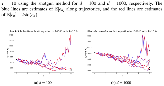
Long horizons become tractable: the method solves the 100- and 1000-dimensional Black–Scholes–Barenblatt equation with T = 10 at relative error within about 2%, a regime where trajectory-matching methods need very many steps.
Extreme dimensions are reachable: tests run up to d = 10000 with local batch M = 64, showing that M can stay far smaller than d.
The residual estimator is gradient-free whenever the PDE coefficients do not depend on $\nabla u$, which removes the $O(d^2)$ Hessian cost that limits PINN for high-dimensional problems.
Because residuals at different collocation points are independent, backward propagation avoids accumulating DNN outputs along trajectories, lowering training cost relative to FBSNN and SDE matching methods.

Reading between the lines

Editorial extensions of the paper, not claims the author makes directly.

A testable extension: applying the same antithetic residual estimator to elliptic or time-independent PDEs, beyond the 1-D Laplace illustration, would show whether the machinery generalizes outside the parabolic setting.
The Section 5.2 heuristic implies that the learning-rate schedule, not just batch size, controls how estimator noise enters the final error; a comparison of constant versus decaying learning rate at fixed M would test this directly.
Because local noise averaging is independent per collocation point, the estimator could be combined with quasi-Monte Carlo or stratified sampling of $\eta$ to reduce the needed batch M; the paper does not explore this.

Share X Bluesky LinkedIn Reddit HN

Signed reviews

No signed human review yet.

Editorial analysis

A structured set of objections, weighed in public.

Desk editor's note, referee report, and a circularity audit.

Desk Editor's Note

read the letter

Short version: the shotgun method is a legitimate incremental contribution. It replaces full-trajectory training in deep FBSDE solvers with coarse trajectory sampling plus a local antithetic residual estimator, and the numerics show real gains: on a 100-d BSB equation, N=10 with M=16 matches SDE matching at N=192, with lower backprop cost; they push to d=10000, T=10. That is worth a referee's time.

What is genuinely new is eqs. (18)-(22): the antithetic average of two one-sided Euler steps gives a single-step residual estimate whose bias is O(Δt) and whose variance is O(1), with the variance reducible by averaging M local samples. That is a clean hybrid of PINN-style residual evaluation and FBSDE data distributions, and it is distinct from the random finite-difference tricks in [11,17]. The paper also deserves credit for testing against exact or high-accuracy references and for openly flagging the L2-loss limitation in Section 5.4.

Now the soft spots. First, the stress-test's central complaint about Appendix A does not land. The appendix writes εΔt, derives Var(εΔt)=O(Δt^2), and that immediately implies Var(ε)=O(1) for the estimator error ε. The notation is sloppy and easy to misread—the paper should have said 'we analyze Δt·ε'—but the claimed bound (20) is not contradicted. The real theoretical gap is Section 5.2. The argument there assumes residuals are linear in θ and that the perturbation is independent of θ, both false in the actual algorithm since the noise is built from ∇²u_θ. The paper calls it non-rigorous, which is honest, but the mechanism that lets M=64 work in d=10000 is still unexplained beyond a toy model and experiments. That is a genuine gap, though not fatal for an engineering contribution.

Second, reproducibility is incomplete. No code is released, only 'available upon request,' and the comparisons are thin: only SDE matching is benchmarked in detail, there are no runtime tables, and the Allen-Cahn case reports a single number without error bars. The d=10000 test is on a different GPU.

Overall, the numerical evidence is credible and the method is practical. The theory is heuristic at the convergence level, and the appendix needs a rewrite for clarity. I'd send it to review and ask for code, a cleaner statement of the variance scaling, and at least one comparison to diffusion loss or DeepMartNet. The stress-test note should not be the basis for a desk reject.

Referee Report

3 major / 6 minor

Summary. The paper introduces a 'shotgun method' for solving high-dimensional parabolic PDEs of the form (1), combining ideas from deep FBSDE formulations and PINNs. Instead of simulating full trajectories at a fine time step, the method draws collocation points from coarsely discretized SDE trajectories and estimates the PDE residual at each point with a local antithetic single-step estimator, Algorithm 1. The residual estimator is averaged over M local samples with local step Δt, while the trajectory step ℓ = T/N can be much larger than Δt. The DNN u_θ(t,x) is trained by minimizing the squared residuals plus a terminal loss, as described in Algorithm 2. Numerical experiments include a 1D Laplace problem, a 100D HJB equation with T = 1 and T = 10, a 100D Allen–Cahn equation, and the Black–Scholes–Barenblatt equation in dimensions up to 10000 and with T = 10. The results are compared with the SDE matching method of [20] and with reference solutions, and the authors claim competitive accuracy at lower backward-propagation cost. The theoretical discussion in Appendix A aims to justify the bias and variance of the residual estimator, and Section 5.2 gives a heuristic explanation for why large residual variance is tolerable during training.

Significance. If the numerical results are taken at face value, the method is a useful practical contribution: it decouples the trajectory discretization from the residual accuracy, which could reduce the cost of long-time high-dimensional problems, and it is tested against external references (closed-form BSB solution, Monte Carlo HJB reference, known Allen–Cahn value). The paper reports reproducible experimental setups and demonstrations up to d = 10000 and T = 10, which is beyond most existing deep FBSDE experiments. The main weakness is theoretical: the proof of the key estimate (20) is stated incorrectly in Eq. (60), its validity is restricted to Δt ≪ 1/d while the experiments use dΔt ≈ 10, and the convergence explanation in Section 5.2 is explicitly heuristic with assumptions not satisfied by the algorithm. These issues do not invalidate the numerical evidence, but they limit the strength of the central claim that the method's coarse-N behavior is understood.

major comments (3)

[Appendix A, Eq. (60)] The displayed expansion is for Δt·ε rather than for ε. With η = √Δt δ, the second term in Eq. (60) is (Δt/2)(δ^T H δ − Tr[H]), whose variance is O(Δt^2); this is Var(Δt·ε), not Var(ε). The corresponding term for ε in Eq. (18) would be (1/(2Δt))η^T H η − (1/2)Tr[H], which has O(1) variance. Thus as written Eq. (60) is inconsistent with Eq. (20), but the inconsistency disappears if the left-hand side is corrected to Δt·ε (or if the right-hand side is divided by Δt). Since Eqs. (67)--(68) then imply Eq. (20), this is a notation error rather than a mathematical contradiction; please fix Eq. (60) and define 'εΔt' explicitly.
[Appendix A (Eqs. (60)-(68)) and §4.4] The proof of (20) assumes ∥η∥ ≪ 1, which for σ of order I requires Δt ≪ 1/d. In the high-dimensional BSB tests (§4.4.1) the paper uses d = 10000 and Δt = 4^{-5}, so dΔt ≈ 9.8 and E∥η∥^4 = d(d+2)Δt^2 is not small; the tail term bound in Eq. (65) is therefore not O(Δt^2) in this regime. Consequently the claims E[ε] = O(Δt) and Var(ε) = O(1) are not established for the parameter values used in the experiments. The authors should either restrict the theoretical statement to Δt ≪ 1/d, replace the Taylor argument with a dimension-aware bound, or provide a numerical measurement of E[ε] and Var(ε) as functions of d at fixed Δt. Without one of these, Eq. (20) does not justify taking M ≪ d in the tested regime.
[§5.2] The explanation of why large-variance residuals are tolerable relies on assumptions that are not satisfied by Algorithm 2: the residuals f_k(θ) are taken to be linear, and the perturbations ε_k^{(n)} are assumed independent of θ. In the shotgun method, the perturbation in Eq. (18) depends on ∇²u_θ through the local samples η, so it is parameter-dependent. The section is explicitly non-rigorous, but the paper should state more clearly that no convergence guarantee is proved for the actual algorithm and that Eq. (58) is only an idealized model. This distinction matters because the abstract and Section 5.1 present the tolerance of coarse N as a feature of the method.

minor comments (6)

[Algorithm 1, line 5] The line 'Sample η ∼ N(0, √Δt I_d)' is not a valid variance specification; it should read η ∼ N(0, Δt I_d) (or state that √Δt is the standard deviation).
[§3.2] The sentence 'the total number of collocation points is (N + 2)M' omits the number of trajectories M1 and the fact that each residual evaluation uses two points x±; please clarify whether this count is per trajectory and how the terminal condition is counted.
[Figure 1] The captions for panels (b) and (c) are swapped relative to the definitions f_2 = sin and f_3 = e^{0.5x} in Section 4.1.
[Remark 1] The citation [4] for the randomized Hessian approximation points to the 1000 Genomes consortium paper; this appears to be an incorrect reference.
[§4.2] The reference solution is computed with 10^5 Monte Carlo samples per (t,x), but no standard deviation of this reference is reported; please include a maximum standard error so the reader can gauge the accuracy of the reference.
[§4.3] The Allen–Cahn test reports only the scalar u_θ(0,x0) and no error curve; please add trajectory errors or a comparison with a reference to make the result quantitative.

Circularity Check

0 steps flagged · score 0.0 of 10

No significant circularity: the shotgun residual estimator is derived from the PDE/FBSDE formulation, and all benchmarks are used only for evaluation, not as fitted targets.

full rationale

I walked the paper's claimed derivation chain. Section 3.1 derives the single-step residual estimator (18) from the FBSDE discretization and a Taylor expansion of the test function v; this is a direct mathematical construction, not a fit to the solution. Algorithm 2 trains u_theta by minimizing the squared residual plus the terminal mismatch, with no term involving the reference values used later for testing. The numerical validations—closed-form Black–Scholes–Barenblatt solution, Monte-Carlo reference for the HJB equation, and the known Allen–Cahn initial value—enter only after training as accuracy checks, so the predictions are not forced by construction. The self-citation to the authors' earlier SDE matching method [20] is used as a baseline for comparison and as a description of an existing scheme, not as a load-bearing theorem; no uniqueness result or prior conclusion is imported to justify the shotgun method. Section 5.2 is explicitly labeled a heuristic, and Appendix A's variance computation appears inconsistent with eq. (20): Appendix A concludes Var(ε_Δt)=O(Δt^2), whereas the paper's claim (20) needs Var(ε)=O(1) for the residual estimator. That is a genuine correctness/rigor concern, but it is not circularity—an unproved or even wrong supporting estimate does not make the derivation equivalent to its inputs. The center of the paper is a new estimator plus experiments, not a derivation whose conclusion is assumed in the premises. Therefore no circular step is present, and the score is 0.

Assumptions & free parameters 0 free parameters · 4 assumptions · 0 invented entities

The method rests on standard FBSDE theory and smoothness assumptions, plus two domain assumptions about sampling adequacy and noisy-training convergence. No free parameters or invented entities are introduced.

assumptions (4)

domain assumption The PDE solution and DNN approximator v are smooth enough for the third-order Taylor expansion in Appendix A.
Used in Appendix A to derive the residual estimator's error statistics; not proven for arbitrary DNNs.
standard math The Pardoux-Peng FBSDE theory provides a unique adapted solution linking the PDE and FBSDE system.
Standard background for deep FBSDE methods.
domain assumption Coarse Euler-Maruyama trajectories with step l produce collocation points whose distribution is adequate for training the residual.
Required so that minimizing the residual on these points yields an accurate solution over the domain; no error bound is given.
domain assumption SGD with the noisy residual loss converges to an accurate solution (heuristic in Section 5.2).
Section 5.2 provides only a linearized, non-rigorous argument; if this fails, the method would not work.

how reviews work

0 comments

Cite this review

Pith. "Pith review of A deep shotgun method for solving high-dimensional parabolic partial differential equations." pith.science (2026). https://pith.science/paper/UTKTEYKH

@misc{pith2026250615481,
  author       = {Pith},
  title        = {Pith review of: A deep shotgun method for solving high-dimensional parabolic partial differential equations},
  year         = {2026},
  howpublished = {\url{https://pith.science/paper/UTKTEYKH}},
  note         = {Machine review of arXiv:2506.15481}
}

read the original abstract

Recent advances in deep learning makes solving parabolic partial differential equations (PDEs) in high dimensional spaces possible via forward-backward stochastic differential equation (FBSDE) formulations. The implementation of most existing methods requires simulating multiple trajectories of stochastic processes with a small step size of time discretization to ensure accuracy, hence having limited performance, especially when solving on a large time interval. To address such issue, we propose a deep "shotgun method" that does not exploit full trajectories, but only utilizes the data distribution of them. Numerical results including examples with dimensionality up to 10000 demonstrate the competitiveness of the proposed shotgun method in both performance and accuracy.

Figures

Figures reproduced from arXiv: 2506.15481 by the authors.

**Figure 2.** Relative errors en(ω) of the 100-dimensional Hamilton-Jacobi-Bellman equation (29) between model predictions and the reference solution along the time interval [0,T] on a single realization of the underlying Brownian motion Wt(ω). (a) T = 1.0 (b) T = 10.0 [PITH_FULL_IMAGE:figures/full_fig_p014_2.png] view at source ↗

**Figure 3.** Predicting Yt trajectories in the FBSDE formulation using trained DNNs. The Xt trajectories are simulated with fine time discretization on a realization of the underling Brownian motion Wt(ω) (same as in [PITH_FULL_IMAGE:figures/full_fig_p014_3.png] view at source ↗

Figures from the paper (6 more)

**Figure 4.** Figure 4: Predicting Yt trajectories in the FBSDE formulation of the 100-D BlackScholes-Barenblatt equation (43) using trained DNNs. The Xt trajectories are simulated with fine time discretization. The red dashed lines are evaluated using u(t,Xt) for reference, and the blue li…

**Figure 5.** Figure 5: Test error en of the 100-D Black-Scholes-Barenblatt equation (43) using the shotgun method with M = 4,16,64 and the SDE matching method [20], respectively. The blue lines are estimates of E[en] along trajectories, and the red lines are estimates of E[en] +2std(en). sup…

**Figure 6.** Figure 6: shows the test errors en in (36) with terminal time T = 1 (and with trajectory discretization steps N = 10) and with dimensionality d = 1000, 2000, 5000 and 100001 , respectively. (a) d = 1000 (b) d = 2000 (c) d = 5000 (d) d = 10000 [PITH_FULL_IMAGE:figures/full_fig_…

**Figure 7.** Figure 7: Predicting Yt trajectories in the FBSDE formulation of the 2000-dimensional BSB equation (43) using trained DNNs. The red dashed lines are evaluated using u(t,Xt) = exp(v(t,Xt)) for reference, and the blue lines are predictions using trained v˜θ (t,Xt). 4.4.2 Case T = …

**Figure 8.** Figure 8: Test error en of the d-dimensional Black-Scholes-Barenblatt equation with T = 10 using the shotgun method for d = 100 and d = 1000, respectively. The blue lines are estimates of E[en] along trajectories, and the red lines are estimates of E[en] +2std(en). (a) d = 100 (…

**Figure 9.** Figure 9: Predicting Yt trajectories in the FBSDE formulation of the Black-ScholesBarenblatt equation (43) with T = 10 using trained DNNs. The red dashed lines are evaluated using u(t,Xt) for reference, and the blue lines are predictions of uθ (t,Xt). where to sample. The shotg…

Review history (2 revisions) →

Discussion (0). Continue with ORCID to comment.

Reference graph

Works this paper leans on

20 extracted references · 15 canonical work pages

[20]

Journal of Computational Physics 470, 111557 (2022)

Zhang, W., Cai, W.: Fbsde based neural network algorithms for high-dimensional quasilinear parabolic pdes. Journal of Computational Physics 470, 111557 (2022)

work page 2022
[1]

Nucleic acids re- search 9(13), 3015–3027 (1981)

Anderson, S.: Shotgun dna sequencing using cloned dnase i-generated fragments. Nucleic acids re- search 9(13), 3015–3027 (1981)

work page 1981
[2]

SOC-MartNet: A Martingale Neural Network for the Hamilton-Jacobi-Bellman Equation without Explicit inf H in Stochastic Optimal Controls

Cai, W., Fang, S., Zhou, T.: Soc-martnet: A martingale neural network for the hamilton- jacobi-bellman equation without explicit inf h in stochastic optimal controls. arXiv preprint arXiv:2405.03169 (2024)

work page Pith review arXiv 2024
[3]

DeepMartNet -- A Martingale Based Deep Neural Network Learning Method for Dirichlet BVPs and Eigenvalue Problems of Elliptic PDEs in R^d

Cai, W., He, A., Margolis, D.: Deepmartnet–a martingale based deep neural network learning method for dirichlet bvp and eigenvalue problems of elliptic pdes. arXiv preprint arXiv:2311.09456 (2023)

work page Pith review arXiv 2023
[4]

Nature526(7571), 68 (2015)

Consortium, .G.P., et al.: A global reference for human genetic variation. Nature526(7571), 68 (2015)

work page 2015
[5]

Proceedings of the National Academy of Sciences 115(34), 8505–8510 (2018)

Han, J., Jentzen, A., E, W.: Solving high-dimensional partial differential equations using deep learn- ing. Proceedings of the National Academy of Sciences 115(34), 8505–8510 (2018)

work page 2018
[6]

Probability, Uncertainty and Quantitative Risk 5(1), 5 (2020)

Han, J., Long, J.: Convergence of the deep bsde method for coupled fbsdes. Probability, Uncertainty and Quantitative Risk 5(1), 5 (2020)

work page 2020
[7]

Neural Networks 176, 106369 (2024)

Hu, Z., Shukla, K., Karniadakis, G.E., Kawaguchi, K.: Tackling the curse of dimensionality with physics-informed neural networks. Neural Networks 176, 106369 (2024). DOI 10.1016/j.neunet. 2024.106369

arXiv 2024

Show all 20 references

[8]

arXiv preprint arXiv:2311.15283 (2023)

Hu, Z., Yang, Z., Wang, Y ., Karniadakis, G.E., Kawaguchi, K.: Bias-variance trade-off in physics- informed neural networks with randomized smoothing for high-dimensional pdes. arXiv preprint arXiv:2311.15283 (2023)

2023 arXiv
[9]

SIAM Journal on Scientific Computing43(6), B1105– B1132 (2021)

Lu, L., Pestourie, R., Yao, W., Wang, Z., Verdugo, F., Johnson, S.G.: Physics-informed neural net- works with hard constraints for inverse design. SIAM Journal on Scientific Computing43(6), B1105– B1132 (2021)

2021
[10]

Journal of Machine Learning 2(1), 31–64 (2023)

N ¨usken, N., Richter, L.: Interpolating between bsdes and pinns: Deep learning for elliptic and parabolic boundary value problems. Journal of Machine Learning 2(1), 31–64 (2023). DOI 10.4208/jml.220416

2023 doi
[11]

arXiv preprint arXiv:2007.10412 (2020)

Oktay, D., McGreivy, N., Aduol, J., Beatson, A., Adams, R.P.: Randomized automatic differentiation. arXiv preprint arXiv:2007.10412 (2020)

2020 arXiv
[12]

Systems & control letters 14(1), 55–61 (1990)

Pardoux, E., Peng, S.: Adapted solution of a backward stochastic differential equation. Systems & control letters 14(1), 55–61 (1990)

1990
[13]

Pardoux, E., Peng, S.: Backward stochastic differential equations and quasilinear parabolic partial dif- ferential equations. In: Stochastic Partial Differential Equations and Their Applications: Proceedings of IFIP WG 7/1 International Conference University of North Carolina ...

2005
[14]

In: Peter Carr Gedenkschrift: Research Advances in Mathematical Finance, pp

Raissi, M.: Forward–backward stochastic neural networks: deep learning of high-dimensional partial differential equations. In: Peter Carr Gedenkschrift: Research Advances in Mathematical Finance, pp. 637–655. World Scientific (2024)

2024
[15]

Journal of Computational physics 378, 686–707 (2019)

Raissi, M., Perdikaris, P., Karniadakis, G.E.: Physics-informed neural networks: A deep learning framework for solving forward and inverse problems involving nonlinear partial differential equa- tions. Journal of Computational physics 378, 686–707 (2019)

2019
[16]

Journal of Machine Learning Re- search 25(248), 1–40 (2024)

Richter, L., Sallandt, L., N ¨usken, N.: From continuous-time formulations to discretization schemes: tensor trains and robust regression for bsdes and parabolic pdes. Journal of Machine Learning Re- search 25(248), 1–40 (2024). URL http://jmlr.org/papers/v25/23-0982.html Deep...

2024
[17]

arXiv preprint arXiv:2310.14168 (2023)

Shukla, K., Shin, Y .: Randomized forward mode of automatic differentiation for optimization algo- rithms. arXiv preprint arXiv:2310.14168 (2023)

2023 arXiv
[18]

Journal of computational physics 375, 1339–1364 (2018)

Sirignano, J., Spiliopoulos, K.: Dgm: A deep learning algorithm for solving partial differential equa- tions. Journal of computational physics 375, 1339–1364 (2018)

2018
[19]

Wang, C., Li, S., He, D., Wang, L.: Is l2 physics informed loss always suitable for training physics informed neural network? Advances in Neural Information Processing Systems35, 8278–8290 (2022)

2022

Pith tools

Reviewed August 15, 2026 · model on record in the stance chip above.

[1] [20]

Journal of Computational Physics 470, 111557 (2022)

Zhang, W., Cai, W.: Fbsde based neural network algorithms for high-dimensional quasilinear parabolic pdes. Journal of Computational Physics 470, 111557 (2022)

work page 2022

[2] [1]

Nucleic acids re- search 9(13), 3015–3027 (1981)

Anderson, S.: Shotgun dna sequencing using cloned dnase i-generated fragments. Nucleic acids re- search 9(13), 3015–3027 (1981)

work page 1981

[3] [2]

SOC-MartNet: A Martingale Neural Network for the Hamilton-Jacobi-Bellman Equation without Explicit inf H in Stochastic Optimal Controls

Cai, W., Fang, S., Zhou, T.: Soc-martnet: A martingale neural network for the hamilton- jacobi-bellman equation without explicit inf h in stochastic optimal controls. arXiv preprint arXiv:2405.03169 (2024)

work page Pith review arXiv 2024

[4] [3]

DeepMartNet -- A Martingale Based Deep Neural Network Learning Method for Dirichlet BVPs and Eigenvalue Problems of Elliptic PDEs in R^d

Cai, W., He, A., Margolis, D.: Deepmartnet–a martingale based deep neural network learning method for dirichlet bvp and eigenvalue problems of elliptic pdes. arXiv preprint arXiv:2311.09456 (2023)

work page Pith review arXiv 2023

[5] [4]

Nature526(7571), 68 (2015)

Consortium, .G.P., et al.: A global reference for human genetic variation. Nature526(7571), 68 (2015)

work page 2015

[6] [5]

Proceedings of the National Academy of Sciences 115(34), 8505–8510 (2018)

Han, J., Jentzen, A., E, W.: Solving high-dimensional partial differential equations using deep learn- ing. Proceedings of the National Academy of Sciences 115(34), 8505–8510 (2018)

work page 2018

[7] [6]

Probability, Uncertainty and Quantitative Risk 5(1), 5 (2020)

Han, J., Long, J.: Convergence of the deep bsde method for coupled fbsdes. Probability, Uncertainty and Quantitative Risk 5(1), 5 (2020)

work page 2020

[8] [7]

Neural Networks 176, 106369 (2024)

Hu, Z., Shukla, K., Karniadakis, G.E., Kawaguchi, K.: Tackling the curse of dimensionality with physics-informed neural networks. Neural Networks 176, 106369 (2024). DOI 10.1016/j.neunet. 2024.106369

arXiv 2024