REVIEW 4 major objections 6 minor 60 references
CNN-Derived Elemental Abundances of LAMOST DR10 Giants: Implications for Galactic Substructures
T0 review · 4 major / 6 minor · reviewed 2026-08-06 · deepseek-v4-flash
Pith's one-line read This paper shows that a CNN can map LAMOST low-resolution spectra of 1.1 million giants to APOGEE-grade abundances, then uses the resulting chemistry to argue that substructure PG1 mixes GSE and thick-disk stars while PG2 is an in-situ…
desk verdict A useful public catalog of 1.1M LAMOST giants with CNN abundances, but the headline precision does not transfer to the full sample and the substructure claims rest on 11 stars. read the letter →
The pith
A machine-rendered reading of the paper's core claim, the machinery that carries it, and where it could break.
The reading
What carries the argument
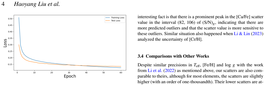
The load-bearing mechanism is label transfer through a convolutional neural network: a three-convolutional-layer, three-fully-connected-layer network that maps 5,000-bin normalized LAMOST spectra to APOGEE DR17 stellar labels, trained on 62,511 common stars. A key preprocessing step is pseudo-normalization by dividing the spectrum by an error-weighted Gaussian-smoothed version, which removes continuum shape while preserving absorption-line information. Dropout is activated at inference time to give per-label uncertainties, following the dropout-as-approximate-Bayesian-inference approach.
What would settle it
Take a sample of very metal-poor giants ([Fe/H] < -2) that were not used in training, run them through the network, and compare with their APOGEE DR17 abundances. If the scatter in C, N, or Ca approaches the paper's own VMP numbers (0.29, 0.40, and 0.48 dex) rather than the overall test-set scatters (0.03 to 0.07 dex), the generalization claim for metal-poor stars collapses; the same check applies to low-S/N stars.
Extended reading notes
Core claim
The central discovery is that low-resolution LAMOST spectra carry enough information to recover APOGEE-grade abundances of C, N, O, Mg, Si, Ca, [α/M], and [M/H] for DR10 giants, and that the resulting chemistry can discriminate between accretion and in-situ origins for halo substructures identified in integral-of-motion space. In the [Mg/Fe]-[Fe/H] plane, the common stars of PG1 split between a high-α, metal-rich clump matching the thick disk and a low-α, low-[Al/Fe] tail matching GSE, while nine of eleven PG2 stars form a tight high-α group with positive [Al/Fe], pointing to an in-situ thin-disk association. The paper frames this as evidence rather than proof, given the small overlap sample, and recommends future data releases and simulations to confirm the origins.
Load-bearing premise
The claim that the catalog is accurate for all 1.1 million giants rests on the assumption that the 62,511 stars with both LAMOST and APOGEE measurements, which supply both the training set and the test set, are representative of the whole population, including the metal-poor and low signal-to-noise stars where the paper itself reports larger scatter.
Editorial extensions
If this is right
- The catalog enables chemical tagging of halo substructures beyond PG1 and PG2, since the derived abundances cover C, N, O, Mg, Si, and Ca for 1.1 million giants.
- [Mg/Fe], [Si/Fe], and [α/M] keep scatter below 0.10 dex even for metal-poor and very metal-poor stars, so these three abundances can be used to study the metal-poor halo where the other element scatters grow larger.
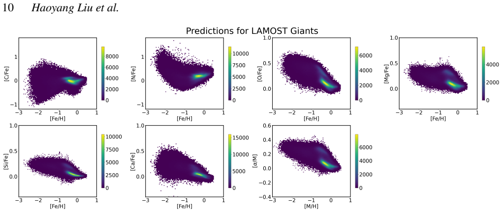
- The high-α thick-disk and low-α thin-disk bimodality appears in all predicted [X/Fe]-[Fe/H] planes, confirming that the network preserves known disk chemistry.
- The predicted Kiel diagram recovers the red clump and the smooth metallicity transition along the giant branch, providing an internal consistency check for the derived parameters.
- If PG1 is a GSE/thick-disk mixture and PG2 is an in-situ thin-disk structure, then integral-of-motion clumps do not map one-to-one onto accreted versus in-situ populations; chemistry is needed to separate the two.
Reading between the lines
- An extension the authors leave implicit is that the same network architecture could be retrained on future LAMOST releases or on medium-resolution spectra, extending the catalog without new survey design.
- The chemical classification of PG1 and PG2 rests on only 11 common stars; a testable extension is to use the catalog's uncertainties to select additional PG1 and PG2 candidates and check whether the bimodality in [Mg/Fe] and [Al/Fe] persists with a larger sample.
- The paper's uncertainty discussion suggests that catalog values outside the reliable ranges listed in Section 3.5 should be treated as flagged rather than as measurements, and a reliability flag column would make this explicit for users.
- The comparisons with previous neural-network and data-driven methods imply that a shared validation set of APOGEE common stars could settle which architecture transfers labels to LAMOST most accurately; the paper does not run such a benchmark.
Editorial analysis
A structured set of objections, weighed in public.
Referee Report
Summary. The authors train a CNN on 62,511 stars common to LAMOST DR10 and APOGEE DR17 to predict T_eff, log g, [Fe/H], [M/H], [C/Fe], [N/Fe], [O/Fe], [Mg/Fe], [Si/Fe], [Ca/Fe], and [alpha/M] for 1,100,858 LAMOST DR10 giants with S/N_g > 10. They report test-set scatters around 50 K, 0.06 dex, and 0.13 dex for T_eff, [Fe/H], and log g, and 0.03–0.07 dex for the elemental abundances, compare with previous label-transfer methods, estimate uncertainties via Monte-Carlo dropout, and release a public catalog. They then cross-match predicted abundances with the PG1 and PG2 substructures from Liu et al. (2024) and argue that PG1 is a GSE/thick-disk mixture and PG2 is an in-situ thin-disk substructure.
Significance. If the precision claims were established on the full 1.1M-star sample, the public catalog would be a valuable resource for Galactic archaeology, complementing APOGEE and GALAH with LAMOST's wide sky coverage. The paper usefully compares with earlier label-transfer methods, quantifies S/N-dependent behavior, and provides per-star uncertainty estimates. However, the current validation is restricted to a random split of APOGEE-LAMOST common stars, and the paper's own metal-poor subsample results show substantially larger scatters, so the catalog-level precision and the substructure interpretation built on it are not yet demonstrated at the claimed level.
major comments (4)
- [Abstract and §3.3 vs §5] The paper reports inconsistent test-set scatter values for the same quantities. The abstract and §3.3 state scatters of 0.07 dex for [C/Fe], 0.05 dex for [N/Fe], 0.05 dex for [O/Fe], 0.04 dex for [Mg/Fe], 0.03 dex for [Si/Fe], 0.04 dex for [Ca/Fe], and 0.06 dex for [M/H], while §5 gives 0.02, 0.03, 0.06, 0.06, 0.01, 0.02, and 0.15 dex for these labels. These are not minor typographical differences: [M/H] changes by 0.09 dex and C/N by 0.03–0.05 dex. Since the precision claims are the central deliverable, the manuscript must adopt one internally consistent set of values and verify them against the test-set calculations.
- [§3.2 and §4.1] The validation design does not support the catalog-level precision claim. The test set is a random 80/20 split of the 62,511 stars that have both LAMOST spectra and APOGEE labels (§3.2), and APOGEE labels were restricted to S/N > 70 and abundance errors < 0.2 dex (§2.1), whereas the catalog includes all LAMOST giants with S/N_g > 10. The manuscript itself reports in §4.1 that for metal-poor stars (−2 < [Fe/H] < −1) and very metal-poor stars ([Fe/H] < −2) the scatters rise to, e.g., 0.15/0.29 dex for C, 0.20/0.40 dex for N, and 0.15/0.48 dex for Ca, versus 0.07/0.05/0.04 dex on the test set. These populations are directly relevant to the halo-substructure claims. The reported test scatters therefore do not validate the precision of the 1.1M-star catalog; please either restrict the precision claims to the common-star-like population or add a representative validation sample that covers the full S/N and metallicity range.
- [§4.2 and Fig. 13] The substructure conclusions rest on very small cross-matches. §4.2 reports 4 LAMOST, 1 APOGEE, and 6 GALAH matches for PG1 and 7 LAMOST, 3 APOGEE, and 1 GALAH matches for PG2, with Figure 13 plotting these together with GSE comparison stars. From these 11 PG1/PG2 common stars, the paper concludes that 'PG2 is highly likely to be an in-situ substructure' and that PG1 is a GSE/thick-disk mixture. With n = 11 and no quantitative mixture model or hypothesis test, this conclusion is not supported. Please rephrase the interpretation as a tentative suggestion and, if possible, add a statistical assessment of how consistent the PG1 and PG2 abundance distributions are with the thick-disk and GSE reference populations.
- [§3.5] The discussion of reliable abundance ranges contains a likely labeling error: the list of ranges appears to include two [C/Fe] intervals (−0.75 to 0.47 dex and −0.24 to 0.82 dex), while no [N/Fe] range is given. Given that §3.5 explicitly discusses the offsets for all elements, this typo affects the usability of the recommended quality cuts and should be corrected.
minor comments (6)
- [§2.1] The word 'acrsecond' should be 'arcsecond'.
- [§3.3] The sentence 'The biases for the elements N, O and Mg are both 0 dex' should read 'are all 0 dex', since three elements are listed.
- [Abstract] The phrase 'The spectral from LAMOST' should be 'The spectra from LAMOST'.
- [Data Availability] The Data Availability section mentions only LAMOST and APOGEE; the catalog URL given in the abstract should also appear here, with a version/date of access.
- [§3.5] In the compiled text some phrases have missing word spaces (e.g., 'comparisonofbetweenpredictionuncertainties' near the end of §3.5); please check the typesetting in the final version.
- [§5] The Summary uses 'uncertainties' for what are elsewhere called 'scatters' (one standard deviation of residuals); please clarify the terminology to avoid conflating random prediction uncertainty with scatter.
Circularity Check
No significant circularity: the CNN predictions are anchored to external APOGEE ground truth, test-set scatters are honest holdout metrics, and the PG1/PG2 substructures were defined from Gaia astrometry in prior work independent of the derived abundances.
full rationale
The core derivation is a label-transfer exercise: a CNN maps LAMOST low-resolution spectra to APOGEE stellar labels, trained on 62,511 common stars whose abundances are external ground truth (Sections 2.1, 3.1). The test-set scatters (Section 3.3) come from a random 80/20 split (Section 3.2), so they are honest holdout statistics, not refits; the catalog predictions for the 1,100,858 giants are genuine extrapolation to stars never used in fitting. The extrapolation is imperfect - Section 4.1 reports 2-10x larger scatters for metal-poor and very metal-poor stars, and the training labels require S/N>70 while the full sample only requires S/N_g>10 - but this is an external-validity/representativeness risk, not a reduction of a prediction to its inputs. No equation defines a predicted quantity from the fitted labels; the dropout-based 'uncertainties' (Section 3.5) are explicitly epistemic, and the paper states they 'do not directly correlate with the offsets between the predicted labels and the APOGEE labels.' The substructure analysis (Section 4.2) uses PG1/PG2 memberships from Liu et al. (2024), a prior paper by overlapping authors, but that catalog was built from Gaia DR3 astrometry in integral-of-motion space (E, L_z, L_perp) via HDBSCAN clustering, i.e., data disjoint from the CNN abundances; the paper also notes LEG was independently identified by Dodd et al. (2024), corroborating the catalog. The abundance-based origin conclusions (GSE/thick-disk mixture for PG1, in-situ thin disk for PG2) therefore combine new chemical information with a pre-existing kinematic classification and do not reduce by construction; no uniqueness theorem or ansatz is imported from the authors' prior work. The bimodality in the [X/Fe]-[Fe/H] planes (Figure 10) is presented as recovery of the known thick/thin-disk pattern, not as a new prediction. Flagged limitations: the Summary quotes numbers inconsistent with the Abstract and Section 3.3 (e.g., [M/H] 0.15 vs 0.06 dex; [alpha/M] 0.05 vs 0.03 dex; C/N/O/Mg/Si/Ca values differ as well), and the PG2 in-situ conclusion rests on only 11 common stars total (4 and 7 LAMOST cross-matches for PG1 and PG2) - the paper itself concedes 'the current sample size is relatively limited.' These are presentation and statistical-strength concerns, not circularity.
Assumptions & free parameters
free parameters (2)
- CNN hyperparameters (kernel size 10, filters 16/8/4, dropout 0.2, learning rate 1e-5, batch size 16, 60 epochs) =
selected via validation MAE
- Smoothing length L in pseudo-normalization =
50 Å
assumptions (3)
- domain assumption APOGEE stellar labels are accurate and transferable to LAMOST spectra as intrinsic properties
- domain assumption The random 80/20 train-test split is representative of the full 1.1M giant population
- domain assumption Pseudo-normalization (Eq. 1-2) removes calibration differences while preserving abundance-sensitive features
Cite this review
Pith. "Pith review of CNN-Derived Elemental Abundances of LAMOST DR10 Giants: Implications for Galactic Substructures." pith.science (2026). https://pith.science/paper/GMNIQSNL
@misc{pith2026250616135,
  author       = {Pith},
  title        = {Pith review of: CNN-Derived Elemental Abundances of LAMOST DR10 Giants: Implications for Galactic Substructures},
  year         = {2026},
  howpublished = {\url{https://pith.science/paper/GMNIQSNL}},
  note         = {Machine review of arXiv:2506.16135}
}
abstract
Stellar parameters and abundances provide crucial insights into stellar and Galactic evolution studies. In this work, we developed a convolutional neural network (CNN) to estimate stellar parameters: effective temperature ($T_{\text{eff}}$), surface gravity (log $g$) and metallicity (both [Fe/H] and [M/H]) as well as six $\alpha$-elements (C, N, O, Mg, Si, Ca) and [$\alpha$/M]. We selected giant stars with \( 3500 \, \text{K} < T_{\text{eff}} < 5500 \, \text{K} \) and \( 0 \, \text{dex} < \log g < 3.6 \, \text{dex} \) from the LAMOST and APOGEE surveys, while requiring (S/N)$_g$ of the LAMOST low-resolution spectra $>$ 10, which leaves 1,100,858 giant stars. The spectral from LAMOST and the labels from APOGEE for 62,511 common stars were used as our training set. The corresponding test set yields scatters 50 K, 0.06 dex and 0.13 dex for $T_{\text{eff}}$, [Fe/H] and log $g$, respectively. For $\alpha$ elements O, Mg, Si and Ca, the scatters are 0.05 dex, 0.04 dex, 0.03 and 0.04 dex, respectively. For C and N elements, the scatters are 0.07 dex and 0.05 dex. For [$\alpha$/M] and [M/H], the scatters are 0.03 dex and 0.06 dex. The mean absolute error (MAE) of most elements are between 0.02 $-$ 0.04 dex. The predicted abundances were cross-matched with previously identified substructures PG1 and PG2, with their origins subsequently analyzed. Finally, the catalog is available at https://nadc.china-vo.org/res/r101529/.
Figures


Figures from the paper (10 more)




Reference graph
Works this paper leans on
-
[1]
Abdurro'uf et al., 2022, @doi [ ] 10.3847/1538-4365/ac4414 , https://ui.adsabs.harvard.edu/abs/2022ApJS..259...35A 259, 35
-
[2]
Agarap A. F., 2018, @doi [arXiv e-prints] 10.48550/arXiv.1803.08375 , https://ui.adsabs.harvard.edu/abs/2018arXiv180308375A p. arXiv:1803.08375
-
[3]
Amarante J. A. S., Debattista V. P., Beraldo e Silva L., Laporte C. F. P., Deg N., 2022, @doi [ ] 10.3847/1538-4357/ac8b0d , https://ui.adsabs.harvard.edu/abs/2022ApJ...937...12A 937, 12
-
[4]
Bailer-Jones C. A. L., Rybizki J., Fouesneau M., Demleitner M., Andrae R., 2021, @doi [ ] 10.3847/1538-3881/abd806 , https://ui.adsabs.harvard.edu/abs/2021AJ....161..147B 161, 147
-
[5]
Belokurov V., Erkal D., Evans N. W., Koposov S. E., Deason A. J., 2018, @doi [ ] 10.1093/mnras/sty982 , https://ui.adsabs.harvard.edu/abs/2018MNRAS.478..611B 478, 611
-
[6]
Belokurov V., Sanders J. L., Fattahi A., Smith M. C., Deason A. J., Evans N. W., Grand R. J. J., 2020, @doi [ ] 10.1093/mnras/staa876 , https://ui.adsabs.harvard.edu/abs/2020MNRAS.494.3880B 494, 3880
-
[7]
Bensby T., Feltzing S., Oey M. S., 2014, @doi [ ] 10.1051/0004-6361/201322631 , https://ui.adsabs.harvard.edu/abs/2014A&A...562A..71B 562, A71
-
[8]
Buder S., et al., 2024, @doi [arXiv e-prints] 10.48550/arXiv.2409.19858 , https://ui.adsabs.harvard.edu/abs/2024arXiv240919858B p. arXiv:2409.19858
Show all 60 references
-
[9]
Cui X.-Q., et al., 2012, @doi [Research in Astronomy and Astrophysics] 10.1088/1674-4527/12/9/003 , https://ui.adsabs.harvard.edu/abs/2012RAA....12.1197C 12, 1197
2012 doi
- [10]
-
[11]
M., et al., 2015, @doi [ ] 10.1093/mnras/stv327 , https://ui.adsabs.harvard.edu/abs/2015MNRAS.449.2604D 449, 2604
De Silva G. M., et al., 2015, @doi [ ] 10.1093/mnras/stv327 , https://ui.adsabs.harvard.edu/abs/2015MNRAS.449.2604D 449, 2604
2015 doi
-
[12]
M., Cassisi S., Fern \'a ndez-Alvar E., Surot F., 2024, @doi [arXiv e-prints] 10.48550/arXiv.2408.13763 , https://ui.adsabs.harvard.edu/abs/2024arXiv240813763D p
Dodd E., Ruiz-Lara T., Helmi A., Gallart C., Callingham T. M., Cassisi S., Fern \'a ndez-Alvar E., Surot F., 2024, @doi [arXiv e-prints] 10.48550/arXiv.2408.13763 , https://ui.adsabs.harvard.edu/abs/2024arXiv240813763D p. arXiv:2408.13763
-
[13]
A., O'Briain T., Bialek S., Kielty C
Fabbro S., Venn K. A., O'Briain T., Bialek S., Kielty C. L., Jahandar F., Monty S., 2018, @doi [ ] 10.1093/mnras/stx3298 , https://ui.adsabs.harvard.edu/abs/2018MNRAS.475.2978F 475, 2978
2018 doi
-
[14]
Fernandes L., et al., 2023, @doi [ ] 10.1093/mnras/stac3543 , https://ui.adsabs.harvard.edu/abs/2023MNRAS.519.3611F 519, 3611
2023 doi
-
[15]
Fuhrmann K., 1998, , https://ui.adsabs.harvard.edu/abs/1998A&A...338..161F 338, 161
1998
- [16]
-
[17]
J., Brook C
Gallart C., Bernard E. J., Brook C. B., Ruiz-Lara T., Cassisi S., Hill V., Monelli M., 2019, @doi [Nature Astronomy] 10.1038/s41550-019-0829-5 , https://ui.adsabs.harvard.edu/abs/2019NatAs...3..932G 3, 932
2019 doi
-
[18]
E., et al., 2016, @doi [ ] 10.3847/0004-6256/151/6/144 , https://ui.adsabs.harvard.edu/abs/2016AJ....151..144G 151, 144
Garc \' a P \'e rez A. E., et al., 2016, @doi [ ] 10.3847/0004-6256/151/6/144 , https://ui.adsabs.harvard.edu/abs/2016AJ....151..144G 151, 144
2016 doi
-
[19]
Gilmore G., Reid N., 1983, @doi [ ] 10.1093/mnras/202.4.1025 , https://ui.adsabs.harvard.edu/abs/1983MNRAS.202.1025G 202, 1025
1983 doi
-
[20]
Gilmore G., et al., 2012, The Messenger, https://ui.adsabs.harvard.edu/abs/2012Msngr.147...25G 147, 25
2012
-
[21]
Guiglion G., et al., 2020, @doi [ ] 10.1051/0004-6361/202038271 , https://ui.adsabs.harvard.edu/abs/2020A&A...644A.168G 644, A168
2020 doi
-
[22]
E., et al., 2006, @doi [ ] 10.1086/500975 , https://ui.adsabs.harvard.edu/abs/2006AJ....131.2332G 131, 2332
Gunn J. E., et al., 2006, @doi [ ] 10.1086/500975 , https://ui.adsabs.harvard.edu/abs/2006AJ....131.2332G 131, 2332
2006 doi
-
[23]
J., et al., 2022, @doi [ ] 10.3847/1538-3881/ac97e9 , https://ui.adsabs.harvard.edu/abs/2022AJ....164..249H 164, 249
Han J. J., et al., 2022, @doi [ ] 10.3847/1538-3881/ac97e9 , https://ui.adsabs.harvard.edu/abs/2022AJ....164..249H 164, 249
2022 doi
-
[24]
Hasselquist S., et al., 2021, @doi [ ] 10.3847/1538-4357/ac25f9 , https://ui.adsabs.harvard.edu/abs/2021ApJ...923..172H 923, 172
2021 doi
-
[25]
H., Massari D., Veljanoski J., Brown A
Helmi A., Babusiaux C., Koppelman H. H., Massari D., Veljanoski J., Brown A. G. A., 2018, @doi [ ] 10.1038/s41586-018-0625-x , https://ui.adsabs.harvard.edu/abs/2018Natur.563...85H 563, 85
2018 doi
-
[26]
Ho A. Y. Q., et al., 2017, @doi [ ] 10.3847/1538-4357/836/1/5 , https://ui.adsabs.harvard.edu/abs/2017ApJ...836....5H 836, 5
2017 doi
-
[27]
Horta D., et al., 2021, @doi [ ] 10.1093/mnras/staa2987 , https://ui.adsabs.harvard.edu/abs/2021MNRAS.500.1385H 500, 1385
2021 doi
-
[28]
Huang Y., et al., 2020, @doi [ ] 10.3847/1538-4365/ab994f , https://ui.adsabs.harvard.edu/abs/2020ApJS..249...29H 249, 29
2020 doi
- [29]
- [30]
-
[31]
W., Bovy J., 2019, @doi [ ] 10.1093/mnras/sty3217 , https://ui.adsabs.harvard.edu/abs/2019MNRAS.483.3255L 483, 3255
Leung H. W., Bovy J., 2019, @doi [ ] 10.1093/mnras/sty3217 , https://ui.adsabs.harvard.edu/abs/2019MNRAS.483.3255L 483, 3255
2019 doi
-
[32]
Li X., Lin B., 2023, @doi [ ] 10.1093/mnras/stad831 , https://ui.adsabs.harvard.edu/abs/2023MNRAS.521.6354L 521, 6354
2023 doi
-
[33]
Li Z., Zhao G., Chen Y., Liang X., Zhao J., 2022, @doi [ ] 10.1093/mnras/stac1959 , https://ui.adsabs.harvard.edu/abs/2022MNRAS.517.4875L 517, 4875
2022 doi
-
[34]
Liu H., Du C., Ye D., Zhang J., Deng M., 2024, @doi [ ] 10.3847/1538-4357/ad8352 , https://ui.adsabs.harvard.edu/abs/2024ApJ...976..161L 976, 161
2024 doi
-
[35]
L., et al., 2015, @doi [Research in Astronomy and Astrophysics] 10.1088/1674-4527/15/8/002 , https://ui.adsabs.harvard.edu/abs/2015RAA....15.1095L 15, 1095
Luo A. L., et al., 2015, @doi [Research in Astronomy and Astrophysics] 10.1088/1674-4527/15/8/002 , https://ui.adsabs.harvard.edu/abs/2015RAA....15.1095L 15, 1095
2015 doi
-
[36]
R., et al., 2017, @doi [ ] 10.3847/1538-3881/aa784d , https://ui.adsabs.harvard.edu/abs/2017AJ....154...94M 154, 94
Majewski S. R., et al., 2017, @doi [ ] 10.3847/1538-3881/aa784d , https://ui.adsabs.harvard.edu/abs/2017AJ....154...94M 154, 94
2017 doi
-
[37]
Martig M., et al., 2016, @doi [ ] 10.1093/mnras/stv2830 , https://ui.adsabs.harvard.edu/abs/2016MNRAS.456.3655M 456, 3655
2016 doi
-
[38]
McWilliam A., Wallerstein G., Mottini M., 2013, @doi [ ] 10.1088/0004-637X/778/2/149 , https://ui.adsabs.harvard.edu/abs/2013ApJ...778..149M 778, 149
2013 doi
-
[39]
C., Vasiliev E., Iorio G., Evans N
Myeong G. C., Vasiliev E., Iorio G., Evans N. W., Belokurov V., 2019, @doi [ ] 10.1093/mnras/stz1770 , https://ui.adsabs.harvard.edu/abs/2019MNRAS.488.1235M 488, 1235
2019 doi
-
[40]
P., Conroy C., Bonaca A., Johnson B
Naidu R. P., Conroy C., Bonaca A., Johnson B. D., Ting Y.-S., Caldwell N., Zaritsky D., Cargile P. A., 2020, @doi [ ] 10.3847/1538-4357/abaef4 , https://ui.adsabs.harvard.edu/abs/2020ApJ...901...48N 901, 48
2020 doi
-
[41]
W., Rix H
Ness M., Hogg D. W., Rix H. W., Ho A. Y. Q., Zasowski G., 2015, @doi [ ] 10.1088/0004-637X/808/1/16 , https://ui.adsabs.harvard.edu/abs/2015ApJ...808...16N 808, 16
2015 doi
-
[42]
Pedregosa F., et al., 2011, Journal of Machine Learning Research, 12, 2825
2011
-
[43]
Steinmetz M., et al., 2006, @doi [ ] 10.1086/506564 , https://ui.adsabs.harvard.edu/abs/2006AJ....132.1645S 132, 1645
2006 doi
-
[44]
Sun T., et al., 2025, @doi [Nature Communications] 10.1038/s41467-025-56550-1 , https://ui.adsabs.harvard.edu/abs/2025NatCo..16.1581S 16, 1581
2025 doi
-
[45]
X., Woosley S
Timmes F. X., Woosley S. E., Weaver T. A., 1995, @doi [ ] 10.1086/192172 , https://ui.adsabs.harvard.edu/abs/1995ApJS...98..617T 98, 617
1995 doi
-
[46]
Ting Y.-S., Conroy C., Rix H.-W., Cargile P., 2019, @doi [ ] 10.3847/1538-4357/ab2331 , https://ui.adsabs.harvard.edu/abs/2019ApJ...879...69T 879, 69
2019 doi
- [47]
-
[48]
Vasini A., Spitoni E., Matteucci F., 2024, @doi [ ] 10.1051/0004-6361/202347603 , https://ui.adsabs.harvard.edu/abs/2024A&A...683A.121V 683, A121
2024 doi
-
[49]
Wang R., et al., 2020, @doi [ ] 10.3847/1538-4357/ab6dea , https://ui.adsabs.harvard.edu/abs/2020ApJ...891...23W 891, 23
2020 doi
-
[50]
Wang C., Huang Y., Yuan H., Zhang H., Xiang M., Liu X., 2022, @doi [ ] 10.3847/1538-4365/ac4df7 , https://ui.adsabs.harvard.edu/abs/2022ApJS..259...51W 259, 51
2022 doi
-
[51]
L., Zhang S., Ting Y.-S., O'Briain T., Lamost Mrs Collaboration 2023, @doi [ ] 10.3847/1538-4365/acce36 , https://ui.adsabs.harvard.edu/abs/2023ApJS..266...40W 266, 40
Wang R., Luo A. L., Zhang S., Ting Y.-S., O'Briain T., Lamost Mrs Collaboration 2023, @doi [ ] 10.3847/1538-4365/acce36 , https://ui.adsabs.harvard.edu/abs/2023ApJS..266...40W 266, 40
2023 doi
-
[52]
306, Statistical Challenges in 21st Century Cosmology
Wu Y., Du B., Luo A., Zhao Y., Yuan H., 2014, in Heavens A., Starck J.-L., Krone-Martins A., eds, IAU Symposium Vol. 306, Statistical Challenges in 21st Century Cosmology. pp 340--342 ( @eprint arXiv 1407.1980 ), @doi 10.1017/S1743921314010825
2014 arXiv
-
[53]
Xiang M., et al., 2019, @doi [ ] 10.3847/1538-4365/ab5364 , https://ui.adsabs.harvard.edu/abs/2019ApJS..245...34X 245, 34
2019 doi
-
[54]
Xiang G., Chen J., Qiu B., Lu Y., 2021, @doi [ ] 10.1088/1538-3873/abd997 , https://ui.adsabs.harvard.edu/abs/2021PASP..133b4504X 133, 024504
2021 doi
-
[55]
Xie J., Bu Y., Liang J., Li H., Wang X., Pan J., 2021, @doi [ ] 10.3847/1538-3881/ac1c7c , https://ui.adsabs.harvard.edu/abs/2021AJ....162..155X 162, 155
2021 doi
-
[56]
Yang C., et al., 2019, @doi [ ] 10.3847/1538-4357/ab2462 , https://ui.adsabs.harvard.edu/abs/2019ApJ...880...65Y 880, 65
2019 doi
-
[57]
Yanny B., et al., 2009, @doi [ ] 10.1088/0004-6256/137/5/4377 , https://ui.adsabs.harvard.edu/abs/2009AJ....137.4377Y 137, 4377
2009 doi
-
[58]
Q., Wang Q
Zhang X., Zhao G., Yang C. Q., Wang Q. X., Zuo W. B., 2019, @doi [ ] 10.1088/1538-3873/ab2687 , https://ui.adsabs.harvard.edu/abs/2019PASP..131i4202Z 131, 094202
2019 doi
-
[59]
Zhang B., Liu C., Deng L.-C., 2020, @doi [ ] 10.3847/1538-4365/ab55ef , https://ui.adsabs.harvard.edu/abs/2020ApJS..246....9Z 246, 9
2020 doi
-
[60]
M., Mao S., 2001, @doi [ ] 10.1086/319832 , https://ui.adsabs.harvard.edu/abs/2001ApJ...551L..85Z 551, L85
Zhao G., Qiu H. M., Mao S., 2001, @doi [ ] 10.1086/319832 , https://ui.adsabs.harvard.edu/abs/2001ApJ...551L..85Z 551, L85
2001 doi
Reviewed August 6, 2026 · model on record in the stance chip above.
Discussion (0). Sign in to comment.