Bounding statistical errors in lattice field theory simulations
Pith reviewed 2026-05-19 09:03 UTC · model grok-4.3
The pith
Upper and lower bounds on the autocorrelation function yield an automatic stopping criterion for unbiased statistical error estimates in lattice Monte Carlo simulations.
A machine-rendered reading of the paper's core claim, the machinery that carries it, and where it could break.
Core claim
By constructing upper and lower bounds on the autocorrelation function, a stopping criterion can be imposed that determines the integration window automatically; the resulting error estimates remain unbiased for both standard Monte Carlo and master-field analyses of lattice field theories.
What carries the argument
Automatic windowing procedure that uses simultaneous upper and lower bounds on the autocorrelation function as a stopping criterion for the integrated autocorrelation time.
Load-bearing premise
Upper and lower bounds on the autocorrelation function can be computed or estimated in practice and produce a stopping rule whose error estimates stay unbiased when moving from toy models to full lattice simulations.
What would settle it
Applying the automatic windowing procedure to a toy model with exactly known variance and finding that the reported error bars differ from the true statistical uncertainty by more than the expected fluctuation.
Figures


read the original abstract
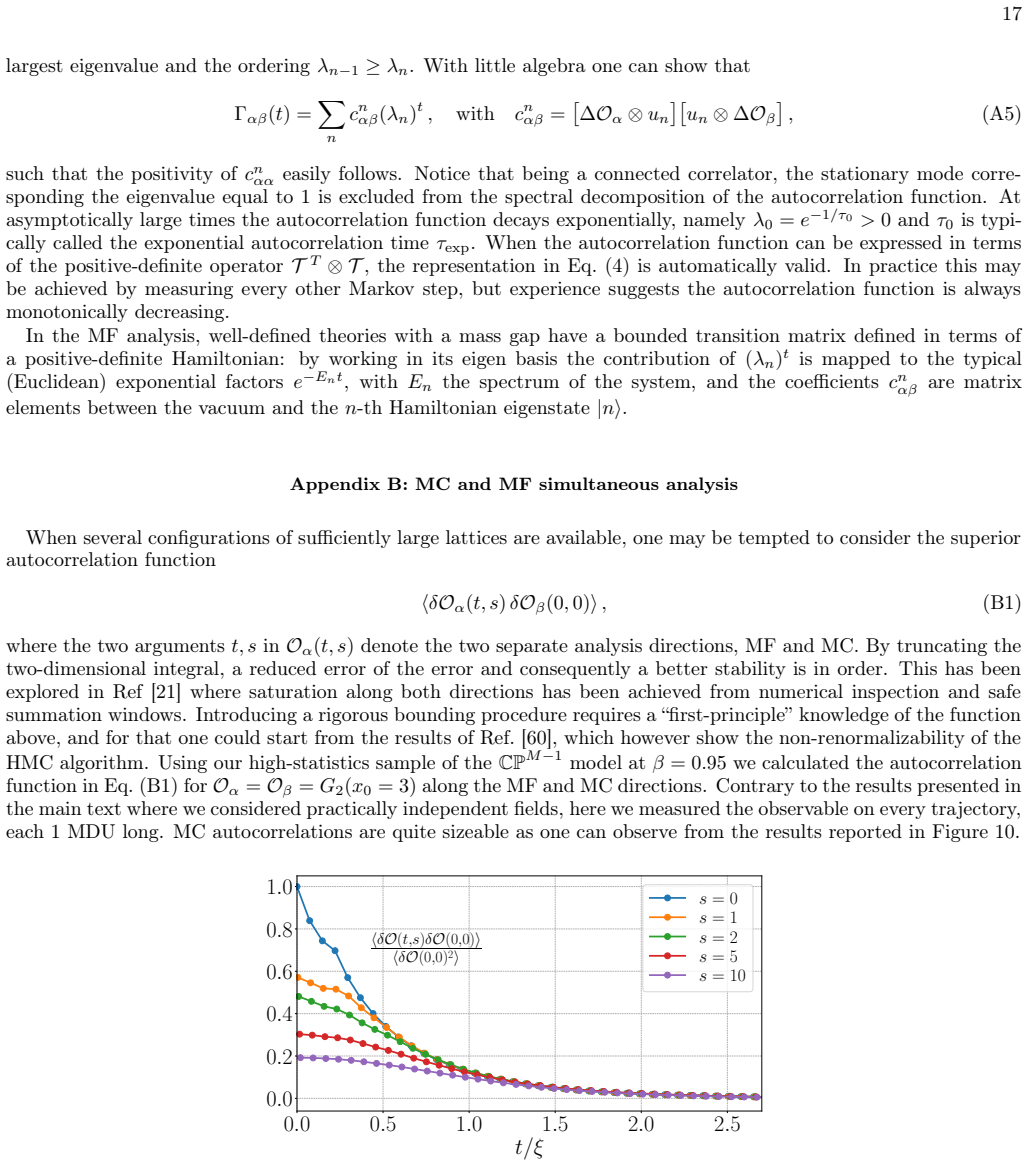
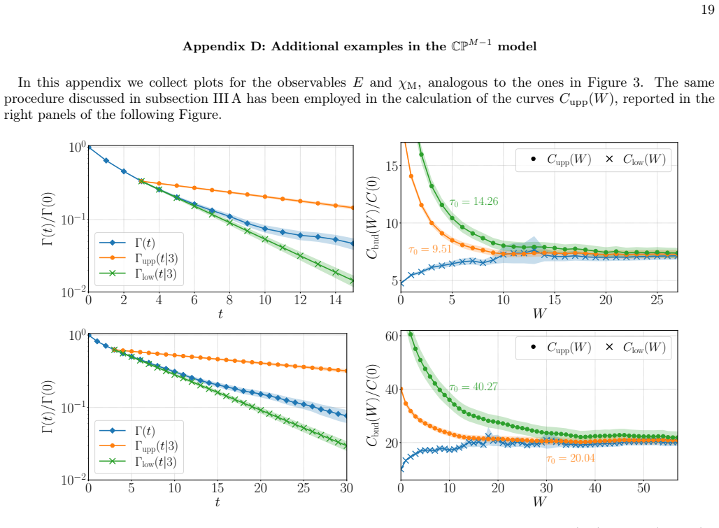
Simulations of strongly interacting lattice field theories are typically performed using Markov chain Monte Carlo algorithms. Therefore estimators of statistical errors must incorporate the effect of autocorrelations by integrating the corresponding autocorrelation function. Since in practical calculations its integral is truncated to a finite window, in this work we propose a stopping criterion based on upper and lower bounds of the autocorrelation function. We examine its application to both traditional Monte Carlo analysis and the recently introduced master-field approach. By leveraging both bounds, we introduce an automatic windowing procedure which we test on numerical simulations of a few simplified toy models.
Editorial analysis
A structured set of objections, weighed in public.
Referee Report
Summary. The paper proposes a stopping criterion for truncating the integrated autocorrelation function in statistical error estimation for lattice field theory Markov chain Monte Carlo simulations. Upper and lower bounds on the autocorrelation function are used to define an automatic windowing procedure, which is examined for both conventional analysis and the master-field approach, with numerical tests performed on simplified toy models.
Significance. If the bounds prove computable and the resulting errors remain unbiased when applied to realistic lattice simulations, the method could offer a systematic improvement over ad-hoc window choices. The manuscript explicitly tests the procedure on toy models, providing a reproducible starting point for assessing its performance.
major comments (1)
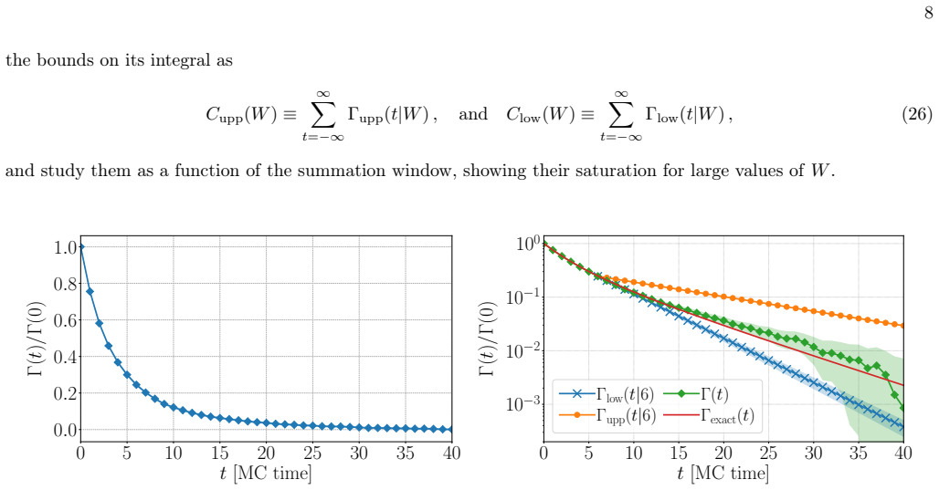
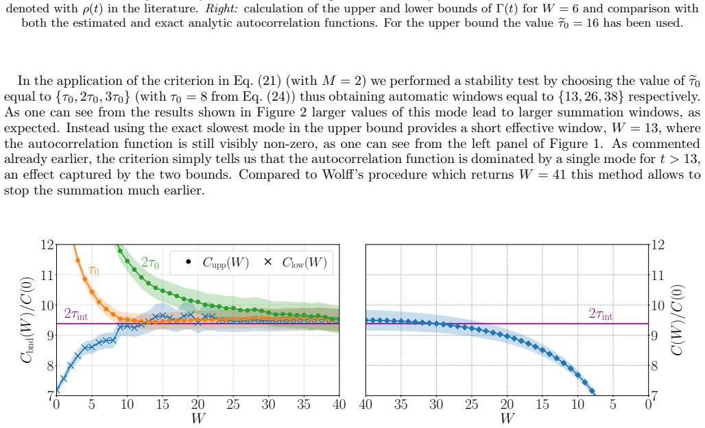
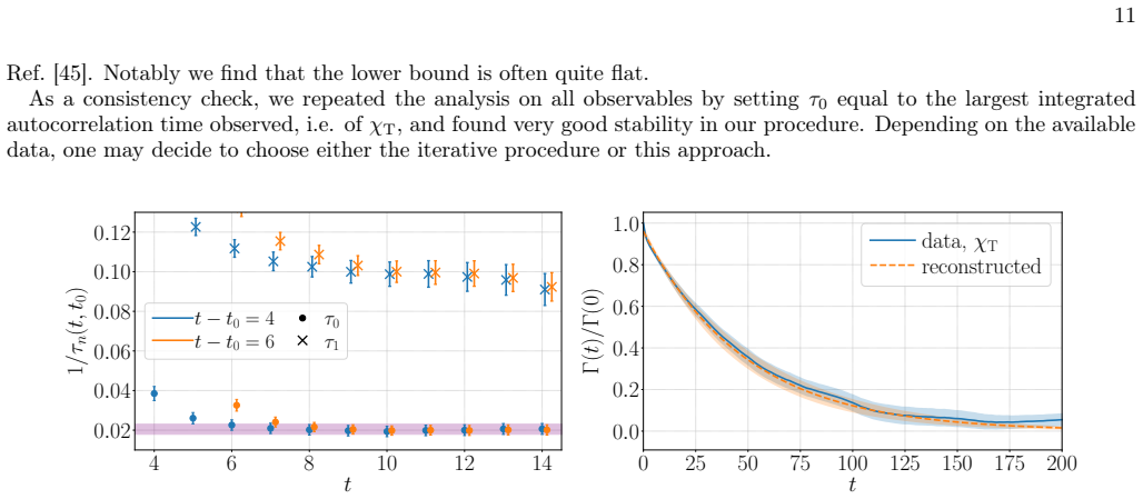
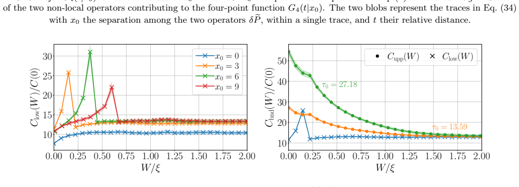
- [§4] §4 (numerical tests on toy models): the central claim is that the bounds enable an automatic windowing procedure yielding unbiased error estimates in lattice field theory simulations, yet all validation is restricted to a few simplified toy models. This leaves open whether the bounds stay sufficiently tight (and the stopping criterion unbiased) for complex actions, gauge fields, or near-critical dynamics referenced in the introduction.
minor comments (1)
- [Methods] The precise construction of the upper and lower bounds (including any assumptions needed for their practical computation) should be stated more explicitly in the methods section.
Simulated Author's Rebuttal
We thank the referee for the careful review and the constructive comment on the scope of our numerical tests. We respond to the major comment below.
read point-by-point responses
-
Referee: [§4] §4 (numerical tests on toy models): the central claim is that the bounds enable an automatic windowing procedure yielding unbiased error estimates in lattice field theory simulations, yet all validation is restricted to a few simplified toy models. This leaves open whether the bounds stay sufficiently tight (and the stopping criterion unbiased) for complex actions, gauge fields, or near-critical dynamics referenced in the introduction.
Authors: We agree that the numerical tests are performed exclusively on simplified toy models. These models were deliberately selected because they permit direct comparison against analytically known results, thereby allowing us to verify that the automatic windowing procedure produces unbiased error estimates in a fully controlled setting. The upper and lower bounds on the autocorrelation function are derived from general properties of stationary Markov processes and do not rely on any assumption of simplicity in the underlying action or dynamics. Consequently the stopping criterion itself is expected to remain valid for the more complex cases mentioned in the introduction. To make this generality clearer, we will add a dedicated paragraph in the revised Section 4 that discusses the anticipated behavior for gauge-field theories and near-critical dynamics, together with a brief outline of how the same bounds-based procedure can be applied in those settings. We view this as a partial revision that addresses the referee’s concern without expanding the computational scope of the present work. revision: partial
Circularity Check
No circularity: new algorithmic stopping criterion derived from proposed bounds, independent of fitted inputs or self-citation chains
full rationale
The paper proposes an automatic windowing procedure that uses upper and lower bounds on the autocorrelation function as a stopping criterion for error estimation in Monte Carlo and master-field analyses. This is presented as a new algorithmic choice rather than a quantity obtained by fitting parameters to the paper's own data or by reducing to prior self-citations. The derivation chain begins from the standard truncation of the integrated autocorrelation and introduces bounds as an external input that can be estimated or computed separately; the resulting procedure is then tested on toy models without the bounds themselves being defined in terms of the window size or error estimate. No step equates a prediction to its own fitted inputs by construction, and the central claim remains self-contained against external benchmarks for the toy-model regime.
Axiom & Free-Parameter Ledger
axioms (1)
- domain assumption Autocorrelation functions in lattice Monte Carlo admit computable upper and lower bounds that can be used for truncation decisions.
Lean theorems connected to this paper
-
IndisputableMonolith/Cost/FunctionalEquation.leanwashburn_uniqueness_aczel unclear?
unclearRelation between the paper passage and the cited Recognition theorem.
We propose a stopping criterion based on upper and lower bounds of the autocorrelation function... Γbnd,α(t|W, τW_eff,α) ≤ Γαα(t) ≤ Γbnd,α(t|W, τ0)
-
IndisputableMonolith/Foundation/ArithmeticFromLogic.leanreality_from_one_distinction unclear?
unclearRelation between the paper passage and the cited Recognition theorem.
the autocorrelation function has an exponentially decreasing behavior... Γαβ(t) = Σ cn_αβ e^{-|t|/τn}
What do these tags mean?
- matches
- The paper's claim is directly supported by a theorem in the formal canon.
- supports
- The theorem supports part of the paper's argument, but the paper may add assumptions or extra steps.
- extends
- The paper goes beyond the formal theorem; the theorem is a base layer rather than the whole result.
- uses
- The paper appears to rely on the theorem as machinery.
- contradicts
- The paper's claim conflicts with a theorem or certificate in the canon.
- unclear
- Pith found a possible connection, but the passage is too broad, indirect, or ambiguous to say the theorem truly supports the claim.
Reference graph
Works this paper leans on
-
[1]
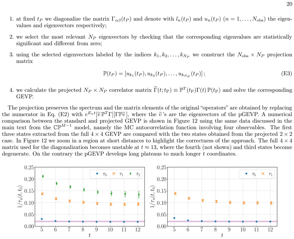
, Nobs) the eigen- values and eigenvectors respectively
at fixedtP we diagonalize the matrixΓαβ(tP ) and denote withln(tP ) and un(tP ) (n = 1, . . . , Nobs) the eigen- values and eigenvectors respectively
-
[2]
we select the most relevantNP eigenvectors by checking that the corresponding eigenvalues are statistically significant and different from zero
-
[3]
, kNP we construct the Nobs × NP projection matrix P(tP ) = [uk1(tP ), uk2(tP ),
using the selected eigenvectors labeled by the indicesk1, k2, . . . , kNP we construct the Nobs × NP projection matrix P(tP ) = [uk1(tP ), uk2(tP ), . . . , ukNP (tP )] ; (E3)
-
[4]
we calculate the projectedNP × NP correlator matrixeΓ(t; tP) ≡ PT (tP)Γ(t) P(tP) and solve the corresponding GEVP. The projection preserves the spectrum and the matrix elements of the original “operators” are obtained by replacing the numerator in Eq. (E2) witheEnt[ev PT Γ][ΓPev ], where theev’s are the eigenvectors of the pGEVP. A numerical comparison be...
-
[5]
T. Aoyamaet al., Phys. Rept.887, 1 (2020), arXiv:2006.04822 [hep-ph]
-
[6]
The anomalous magnetic moment of the muon in the Standard Model: an update
R. Alibertiet al., (2025), arXiv:2505.21476 [hep-ph]
work page internal anchor Pith review Pith/arXiv arXiv 2025
-
[7]
Critical slowing down of topological modes
L. Del Debbio, G. M. Manca, and E. Vicari, Phys. Lett. B594, 315 (2004), arXiv:hep-lat/0403001
work page internal anchor Pith review Pith/arXiv arXiv 2004
- [8]
-
[9]
Monte Carlo errors with less errors
U. Wolff (ALPHA), Comput. Phys. Commun. 156, 143 (2004), [Erratum: Comput. Phys. Commun.176,383(2007)], arXiv:hep-lat/0306017 [hep-lat]
work page internal anchor Pith review Pith/arXiv arXiv 2004
-
[10]
Critical slowing down and error analysis in lattice QCD simulations
S. Schaefer, R. Sommer, and F. Virotta (ALPHA), Nucl. Phys. B845, 93 (2011), arXiv:1009.5228 [hep-lat]
work page internal anchor Pith review Pith/arXiv arXiv 2011
-
[11]
288,108750(2023),arXiv:2209.14371 [hep-lat]
F.Joswig, S.Kuberski, J.T.Kuhlmann, andJ.Neuendorf,Comput.Phys.Commun. 288,108750(2023),arXiv:2209.14371 [hep-lat]
-
[12]
Automatic differentiation for error analysis of Monte Carlo data
A. Ramos, Comput. Phys. Commun.238, 19 (2019), arXiv:1809.01289 [hep-lat]
work page internal anchor Pith review Pith/arXiv arXiv 2019
- [13]
-
[14]
M. Bruno and R. Sommer, Comput. Phys. Commun.285, 108643 (2023), arXiv:2209.14188 [hep-lat]
- [15]
-
[16]
C. Kelly and T. Wang, PoSLA TTICE2019, 129 (2019), arXiv:1911.04582 [hep-lat]
-
[17]
B. Efron, The Jackknife, the Bootstrap and Other Resampling Plans(Society for Industrial and Applied Mathematics, Philadelphia, 1982). 21
work page 1982
-
[18]
M. H. Quenouille, The Annals of Mathematical Statistics20, 355 (1949)
work page 1949
-
[19]
Tukey, Annals of Mathematical Statistics29, 614 (1958)
J. Tukey, Annals of Mathematical Statistics29, 614 (1958)
work page 1958
- [20]
- [21]
-
[22]
L. Giusti and M. Lüscher, Eur. Phys. J. C79, 207 (2019), arXiv:1812.02062 [hep-lat]
-
[23]
P. Fritzsch, J. Bulava, M. Cè, A. Francis, M. Lüscher, and A. Rago, PoSLA TTICE2021, 465 (2022), arXiv:2111.11544 [hep-lat]
- [24]
-
[25]
T. Blumet al.(RBC, UKQCD), Phys. Rev. D108, 054507 (2023), arXiv:2301.08696 [hep-lat]
- [26]
- [27]
-
[28]
Slope and curvature of the hadron vacuum polarization at vanishing virtuality from lattice QCD
S. Borsanyi, Z. Fodor, T. Kawanai, S. Krieg, L. Lellouch, R. Malak, K. Miura, K. K. Szabo, C. Torrero, and B. Toth, Phys. Rev. D96, 074507 (2017), arXiv:1612.02364 [hep-lat]
work page internal anchor Pith review Pith/arXiv arXiv 2017
-
[29]
S. Yamamoto, P. Boyle, T. Izubuchi, L. Jin, C. Lehner, and N. Matsumoto, PoS LA TTICE2024, 034 (2025), arXiv:2502.05452 [hep-lat]
-
[30]
Schwarz-preconditioned HMC algorithm for two-flavour lattice QCD
M. Luscher, Comput. Phys. Commun.165, 199 (2005), arXiv:hep-lat/0409106
work page internal anchor Pith review Pith/arXiv arXiv 2005
- [31]
-
[32]
S. R. Sharpe, inWorkshop on Perspectives in Lattice QCD(2006) arXiv:hep-lat/0607016
work page internal anchor Pith review Pith/arXiv arXiv 2006
- [33]
-
[34]
T. Blumet al.(RBC, UKQCD), Phys. Rev. Lett.134, 201901 (2025), arXiv:2410.20590 [hep-lat]
-
[35]
D. Djukanovic, G. von Hippel, S. Kuberski, H. B. Meyer, N. Miller, K. Ottnad, J. Parrino, A. Risch, and H. Wittig, JHEP 04, 098 (2025), arXiv:2411.07969 [hep-lat]
-
[36]
Bazavovet al., (2024), arXiv:2412.18491 [hep-lat]
A. Bazavovet al., (2024), arXiv:2412.18491 [hep-lat]
- [37]
-
[38]
On the generalized eigenvalue method for energies and matrix elements in lattice field theory
B. Blossier, M. Della Morte, G. von Hippel, T. Mendes, and R. Sommer, JHEP04, 094 (2009), arXiv:0902.1265 [hep-lat]
work page internal anchor Pith review Pith/arXiv arXiv 2009
- [39]
- [40]
- [41]
-
[42]
P. A. Boyle, G. Cossu, A. Yamaguchi, and A. Portelli, PoSLA TTICE 2015, 023 (2016)
work page 2015
-
[43]
Grid Python Toolkit (GPT), 2024-10,
C. Lehner, M. Bruno, D. Richtmann, M. Schlemmer, R. Lehner, D. Knüttel, T. Wurm, L. Jin, S. Bürger, A. Hackl, and A. Klein, “Grid Python Toolkit (GPT), 2024-10,” (2024)
work page 2024
- [44]
- [45]
- [46]
-
[47]
P. Di Vecchia, A. Holtkamp, R. Musto, F. Nicodemi, and R. Pettorino, Nucl. Phys. B190, 719 (1981)
work page 1981
- [48]
-
[49]
G. P. Engel and S. Schaefer, Comput. Phys. Commun.182, 2107 (2011), arXiv:1102.1852 [hep-lat]
work page internal anchor Pith review Pith/arXiv arXiv 2011
-
[50]
Monte Carlo simulation of lattice ${\rm CP}^{N-1}$ models at large N
E. Vicari, Phys. Lett. B309, 139 (1993), arXiv:hep-lat/9209025
work page internal anchor Pith review Pith/arXiv arXiv 1993
-
[51]
Worm Algorithm for CP(N-1) Model
T. Rindlisbacher and P. de Forcrand, Nucl. Phys. B918, 178 (2017), arXiv:1610.01435 [hep-lat]
work page internal anchor Pith review Pith/arXiv arXiv 2017
-
[52]
Precision study of critical slowing down in lattice simulations of the CP^{N-1} model
J. Flynn, A. Juttner, A. Lawson, and F. Sanfilippo, (2015), arXiv:1504.06292 [hep-lat]
work page internal anchor Pith review Pith/arXiv arXiv 2015
-
[53]
Fighting topological freezing in the two-dimensional CP$^{N-1}$ model
M. Hasenbusch, Phys. Rev. D96, 054504 (2017), arXiv:1706.04443 [hep-lat]
work page internal anchor Pith review Pith/arXiv arXiv 2017
- [54]
-
[55]
K. G. Wilson, Phys. Rev. D10, 2445 (1974)
work page 1974
-
[56]
Properties and uses of the Wilson flow in lattice QCD
M. Lüscher, JHEP08, 071 (2010), [Erratum: JHEP 03, 092 (2014)], arXiv:1006.4518 [hep-lat]
work page internal anchor Pith review Pith/arXiv arXiv 2010
-
[57]
Trivializing maps, the Wilson flow and the HMC algorithm
M. Luscher, Commun. Math. Phys.293, 899 (2010), arXiv:0907.5491 [hep-lat]
work page internal anchor Pith review Pith/arXiv arXiv 2010
-
[58]
Perturbative analysis of the gradient flow in non-abelian gauge theories
M. Luscher and P. Weisz, JHEP02, 051 (2011), arXiv:1101.0963 [hep-th]
work page internal anchor Pith review Pith/arXiv arXiv 2011
-
[59]
M. Cè, C. Consonni, G. P. Engel, and L. Giusti, Phys. Rev. D92, 074502 (2015), arXiv:1506.06052 [hep-lat]
work page internal anchor Pith review Pith/arXiv arXiv 2015
-
[60]
Topological susceptibility and the sampling of field space in $N_f=2$ lattice QCD simulations
M. Bruno, S. Schaefer, and R. Sommer (ALPHA), JHEP08, 150 (2014), arXiv:1406.5363 [hep-lat]
work page internal anchor Pith review Pith/arXiv arXiv 2014
-
[61]
A. Athenodorou and M. Teper, JHEP11, 172 (2020), arXiv:2007.06422 [hep-lat]
-
[62]
Computational Strategies in Lattice QCD
M. Luscher, inLes Houches Summer School: Session 93: Modern perspectives in lattice QCD: Quantum field theory and high performance computing(2010) pp. 331–399, arXiv:1002.4232 [hep-lat]
work page internal anchor Pith review Pith/arXiv arXiv 2010
- [63]
-
[64]
Non-renormalizability of the HMC algorithm
M. Luscher and S. Schaefer, JHEP04, 104 (2011), arXiv:1103.1810 [hep-lat]
work page internal anchor Pith review Pith/arXiv arXiv 2011
-
[65]
H. E. Haber, I. Hinchliffe, and E. Rabinovici, Nucl. Phys. B172, 458 (1980)
work page 1980
- [66]
- [67]
-
[68]
T. Blum et al. (RBC, UKQCD), Phys. Rev. D 107, 094512 (2023), [Erratum: Phys.Rev.D 108, 039902 (2023)], arXiv:2301.09286 [hep-lat]
discussion (0)
Sign in with ORCID, Apple, or X to comment. Anyone can read and Pith papers without signing in.