REVIEW 3 major objections 6 minor 45 references
Bounds-constrained finite element approximation of time-dependent partial differential equations
T0 review · 3 major / 6 minor · reviewed 2026-08-15 · deepseek-v4-flash
Pith's one-line read Rewriting collocation time-steppers in the Bernstein basis makes bounds constraints hold uniformly in time while preserving high-order accuracy.
desk verdict A genuinely useful Bernstein-basis reformulation of collocation RK that enforces bounds uniformly in time, but the high-order claim is unproven and the convergence tests happen to avoid the one configuration where the method may lose order. read the letter →
The pith
A machine-rendered reading of the paper's core claim, the machinery that carries it, and where it could break.
The reading
What carries the argument
The load-bearing object is the Bernstein-form reformulation of the collocating polynomial. On each time interval, the collocation polynomial $u(t_n+\tau k)$ is written as $\sum_{j=0}^s Z_j b_j(\tau)$ in the Bernstein basis of degree $s$, related to the stage values by the Bernstein-Vandermonde matrix $V_{ij}=b_j(c_i)$. Replacing the stage-coupled variational equations by a variational inequality over coefficient-bounded Bernstein polynomials makes the convex hull property do the work: with all $Z_j$ in the interval $[m,M]$, the polynomial's values lie in $[m,M]$ for all $\tau\in[0,1]$. The update is then taken by evaluating the last Bernstein coefficient (or the full polynomial), so the constraint transfers to the next time level.
What would settle it
Construct a heat-equation problem whose exact solution has negative Bernstein coefficients on coarse meshes (e.g., a localized smooth bump with steep gradients) and measure the L2 error at t=1 under refinement with k=1/N. If the error stops decreasing at the scheme's nominal order once the active-set boundary is hit, the formal high-order claim fails.
Extended reading notes
Core claim
The central claim is that a collocation Runge-Kutta method can be reorganized so that the unknowns are the Bernstein coefficients of its collocating polynomial rather than stage values. When the stage equations are replaced by variational inequalities over the set of polynomials whose Bernstein coefficients lie in the desired interval, the convex hull property of the Bernstein basis implies the entire polynomial—hence the numerical solution at every time between steps—satisfies the bounds. For stiffly accurate schemes the update is simply the last Bernstein coefficient; for non-stiffly accurate schemes the Bernstein evaluation gives the update directly, so the uniform bound also reaches the new time level. The paper further shows how the same reformulation handles collocation methods with a node at the left endpoint through a confluent Bernstein-Vandermonde system. Numerical tests for all four basis combinations (Lagrange or Bernstein in space, Lagrange or Bernstein in time) show that only the Bernstein-in-time versions avoid constraint violations between collocation nodes.
Load-bearing premise
The load-bearing assumption is that the variational inequality over Bernstein-coefficient-bounded polynomials preserves the formal convergence order of the underlying unconstrained collocation method; the paper demonstrates this order numerically but provides no proof.
Editorial extensions
If this is right
- Four method variants are obtained by choosing Lagrange or Bernstein bases in space and in time; only variants with Bernstein in time guarantee uniform-in-time bounds, and only those with Bernstein in space guarantee uniform-in-space bounds.
- For schemes that are not stiffly accurate, such as Gauss-Legendre, the Bernstein reformulation still produces a bound-respecting update, whereas the Lagrange stage-constrained version can violate bounds at the new time level.
- The Cahn-Hilliard tests with a logarithmic potential run without regularizing the singular term and without a step-size restriction tied to the bound, provided the solver's linearization uses a regularized logarithm.
- Newton-type variational-inequality solvers need only a small number of iterations per step, independent of mesh size, across all tested configurations.
Reading between the lines
- The Bernstein reformulation should transfer to other stage-based integrators with polynomial representations, such as discontinuous Galerkin time-stepping, where a control-coefficient constraint would similarly give a uniform-in-time guarantee.
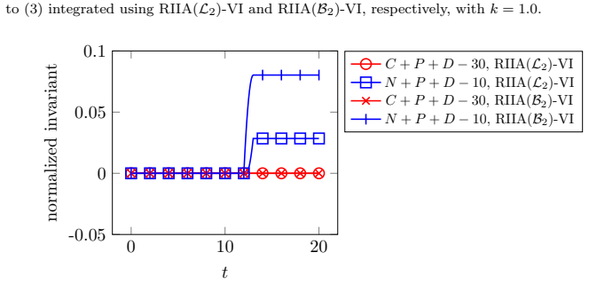
- The small drift in linear invariants seen in the phytoplankton test suggests adding equality constraints for invariants to the feasible set; the paper notes such a set remains closed and convex, so an augmented solver variant is a natural testable extension.
- A convergence proof would likely combine the nodally bound-preserving analysis of the Lagrange case with a Bernstein approximation error bound; until then, the method's reach rests on the observed numerical rates.
Signed reviews
Editorial analysis
A structured set of objections, weighed in public.
Referee Report
Summary. The paper develops bounds-constrained finite element approximations for time-dependent PDEs by combining collocation-type Runge-Kutta methods with variational inequalities. The main novelty is a reformulation of the collocation scheme in the Bernstein basis, so that enforcing bounds on Bernstein coefficients of the collocating polynomial yields uniform-in-time bound satisfaction via the convex hull property. Four method variants are described, depending on whether the spatial finite element space and the temporal collocation polynomial are represented in Lagrange or Bernstein form. Numerical experiments cover a phytoplankton ODE model, the heat equation, and the logarithmic Cahn-Hilliard equation. The authors claim formally high order in both space and time, supported by numerical convergence tests, while explicitly stating in Section 5 that convergence theory is lacking.
Significance. The uniform-in-time bound enforcement mechanism is a clean and useful contribution: the Bernstein reformulation of the stage equations is non-obvious, and the convex hull property gives a rigorous, parameter-free guarantee that the computed solution respects the bounds throughout each time interval. The four-way classification of space/time basis choices is pedagogically and practically useful, and the Cahn-Hilliard experiments with a logarithmic potential show that the approach can handle singular nonlinearities with modest Newton iteration counts. However, the high-order convergence claim is not backed by analysis, and the numerical evidence in Section 4.2.1 is built around a manufactured solution whose zero set is aligned with the mesh. The paper is transparent about the missing theory, but the advertised 'formally high order' claim currently outruns the evidence.
major comments (3)
- [Section 4.2.1, Eq. (46), Figures 6-7] The convergence tests use the exact solution u = e^{-t} cos^2(2πx) sin^2(2πy), whose zero curves are the lines x=1/4, 3/4 and y=0, 1/2, 1. For the uniform N x N mesh with N=4,8,16,..., every zero curve is exactly a mesh line, so each element has the zero set only on its boundary. The Bernstein-coefficient feasible set defined in Section 3.3, Eq. (21), is a strict subset of the bounds-respecting members of the finite element space: a nonnegative polynomial whose zero set crosses an element interior cannot be represented with nonnegative Bernstein coefficients, and the distance from such a local profile to the nonnegative-coefficient cone is O(1) relative to h^2, independent of polynomial degree. Consequently the reported O(h^3) and O(h^4) rates in Figures 6-7 do not test the worst case for the constrained Bernstein space and do not support generic high-order convergence. The authors should add convergence studies with a zero set that crosses element interiors (e.g., a rotated mesh or a solution with a curved zero set) and either prove the high-order claim or substantially qualify it.
- [Introduction and Section 5] The paper cites Bolley and Crouzeix [9] for the statement that a method preserving positivity uniformly in the time step size cannot exceed first order, but then claims high-order methods with uniform-in-time bounds. This apparent tension is not reconciled anywhere in the manuscript. The variational inequality formulation is nonlinear, so the classical linear barrier may not apply, but the authors should explain precisely which hypothesis of the Bolley-Crouzeix result fails for the proposed scheme. Without this discussion, the core claim of high-order accuracy with uniform bounds remains internally inconsistent on its face.
- [Section 5] The manuscript explicitly states 'we lack convergence theory for this method.' This is not by itself an error, but it is a load-bearing admission: the abstract and introduction advertise formally high order methods in both space and time, and the only support is the numerical study of Section 4.2.1, which, as noted above, uses an aligned zero set. The authors should provide a convergence analysis for the stage variational inequality, at least for the linear heat equation, or revise the claims to describe the method as high-order in the unconstrained regime with a uniform bounds guarantee whose interaction with accuracy remains open.
minor comments (6)
- [Section 3.4, Eq. (30)] The symbol v_i is used both for the test function in the inner product and for the i-th component of the vector v in the Bernstein-Vandermonde partition; please rename one of them (for example, use w_i for the test function).
- [Section 3.4, Eqs. (44)-(45)] The Bernstein basis functions are written as b_i^{s+1}(τ) although the collocating polynomial has degree s and therefore has s+1 Bernstein basis functions; the superscript should be s, not s+1.
- [Section 4.2.1] The text says 'optimal convergence rates as k decreases' while the figures plot error against N with k = 1/N; please state the relationship k = 1/N explicitly in the caption or text.
- [Table 1] The numerical entries contain inconsistent spacing (e.g., '1 .5' and '2 .3'), which makes the table difficult to read; please reformat it.
- [Section 4.1, Figure 5 caption] The caption uses 'RIIA(P2)-VI' with an undefined placeholder P; please use the concrete notation L2 or B2 as in the text.
- [Section 4.3] The regularized logarithm is introduced only for computing the Jacobian in the linear solves; please clarify that the residual (and hence the converged solution) is based on the unregularized potential, or if the residual is also regularized, explain the effect on the reported bounds and energy decay.
Circularity Check
No significant circularity: the uniform bounds guarantee is a direct convex-hull consequence of the Bernstein basis, and the numerical convergence tests are illustrative rather than fitted predictions.
full rationale
The paper's central claim—that the Bernstein-form collocation method enforces bounds uniformly in time—is not derived from an input that already contains the conclusion. It follows immediately from the convex hull property of Bernstein polynomials (Section 3.3, Eq. (22) and discussion), which is standard external mathematics. The reformulation in Section 3.4 is an algebraic change of variables: Eq. (26)–(29) relate Lagrange node values Y to Bernstein coefficients Z through the Bernstein–Vandermonde matrix, and the variational inequality (43) is posed on the coefficient constraints by design. The paper explicitly acknowledges this: "By construction, (23) can only produce solutions for which the discretized Runge-Kutta stages satisfy the bounds constraint." This is a design guarantee, not a hidden fit or a prediction derived from a definition. No parameter is fitted to data and then renamed as a prediction. The high-order accuracy claim is explicitly qualified as formal: Section 5 states "we lack convergence theory for this method," and the convergence rates in Section 4.2.1 are numerical illustrations using a manufactured solution, not calibrated outputs. The self-citation [30] is prior work on stationary problems and is presented as a foundation with its own open question ("theoretical convergence rates are still an open question"); the time-dependent Bernstein-collocation extension is derived in this paper rather than assumed from that citation. A possible order-reduction obstruction when a zero curve crosses element interiors would be a correctness or robustness limitation, not circularity, because it does not make the derivation depend on its own conclusion. Overall, the derivation is self-contained: the bound guarantee is a direct mathematical consequence, and the numerical experiments are evidence, not fitted inputs.
Assumptions & free parameters
free parameters (2)
- delta_b (Cahn-Hilliard constraint margin) =
1e-8
- delta_reg (regularized logarithm threshold) =
0.001
assumptions (5)
- standard math Bernstein polynomials form a nonnegative partition of unity and satisfy the convex hull property.
- standard math Continuous collocation methods can be expressed as Runge-Kutta methods.
- domain assumption The variational inequality stage problems (23) and (43) have solutions for the nonlinear operators considered.
- ad hoc to paper Bernstein-coefficient-constrained feasible sets preserve the formal order of the underlying Runge-Kutta method.
- domain assumption The analytical Cahn-Hilliard solution remains in (-1,1) a.e. for all t > 0.
Cite this review
Pith. "Pith review of Bounds-constrained finite element approximation of time-dependent partial differential equations." pith.science (2026). https://pith.science/paper/NTDNVLDH
@misc{pith2026250617464,
  author       = {Pith},
  title        = {Pith review of: Bounds-constrained finite element approximation of time-dependent partial differential equations},
  year         = {2026},
  howpublished = {\url{https://pith.science/paper/NTDNVLDH}},
  note         = {Machine review of arXiv:2506.17464}
}
read the original abstract
Finite element methods provide accurate and efficient methods for the numerical solution of partial differential equations by means of restricting variational problems to finite-dimensional approximating spaces. However, they do not guarantee enforcement of bounds constraints inherent in the original problem. Previous work enforces these bounds constraints by replacing the variational equations with variational inequalities. We extend this approach to collocation-type Runge-Kutta methods for time-dependent problems, obtaining (formally) high order methods in both space and time. By using a novel reformulation of the collocation scheme, we can guarantee that the bounds constraints hold uniformly in time. Numerical examples for a model of phytoplankton growth, the heat equation, and the Cahn-Hilliard system are given.
Figures


Figures from the paper (13 more)



Reference graph
Works this paper leans on
-
[9]
Catherine Bolley and Michel Crouzeix. Conservation de la positivit´ e lors de la discr´ etisation des probl` emes d’´ evolution paraboliques.RAIRO. Analyse num´ erique, 12(3):237–245, 1978
work page 1978
-
[1]
Razan Abu-Labdeh, Scott MacLachlan, and Patrick E. Farrell. Monolithic multigrid for implicit Runge-Kutta discretizations of incompressible fluid flow. Journal of Computational Physics , 478:111961, 2023
work page 2023
-
[2]
ParaView: An end-user tool for large data visualization
James Ahrens, Berk Geveci, and Charles Law. ParaView: An end-user tool for large data visualization. In Visualization Handbook. Elesvier, 2005. ISBN 978-0123875822
2005
-
[3]
Douglas N. Arnold, Richard S. Falk, and Ragnar Winther. Geometric decompositions and local bases for spaces of finite element differential forms. Computer Methods in Applied Mechanics and Engineering , 198(21- 26):1660–1672, 2009
work page 2009
-
[4]
Satish Balay, Shrirang Abhyankar, Mark F. Adams, Steven Benson, Jed Brown, Peter Brune, Kris Buschelman, Emil Constantinescu, Lisandro Dalcin, Alp Dener, Victor Eijkhout, Jacob Faibussowitsch, William D. Gropp, V’aclav Hapla, Tobin Isaac, Pierre Jolivet, Dmitry Karpeev, Di- nesh Kaushik, Matthew G. Knepley, Fande Kong, Scott Kruger, Dave A. May, Lois Curf...
work page 2023
-
[5]
Gropp, Lois Curfman McInnes, and Barry F
Satish Balay, William D. Gropp, Lois Curfman McInnes, and Barry F. Smith. Efficient management of parallelism in object oriented numerical software libraries. In E. Arge, A. M. Bruaset, and H. P. Langtangen, editors, Modern Software Tools in Scientific Computing, pages 163–202. Birkh¨ auser Press, 1997
work page 1997
-
[6]
Gabriel R. Barrenechea, Emmanuil H. Georgoulis, Tristan Pryer, and An- dreas Veeser. A nodally bound-preserving finite element method. IMA Journal of Numerical Analysis , 44(4):2198–2219, 2024
work page 2024
-
[7]
R. K. Beatson. Restricted range approximation by splines and variational inequalities. SIAM Journal on Numerical Analysis , 19(2):372–380, 1982
work page 1982
Show all 45 references
-
[8]
Positivity-preserving methods for ordinary differential equations
Sergio Blanes, Arieh Iserles, and Shev Macnamara. Positivity-preserving methods for ordinary differential equations. ESAIM: Mathematical Mod- elling and Numerical Analysis , 56(6):1843–1870, 2022
2022
-
[10]
A second-order, unconditionally positive, mass-conserving integration scheme 27 for biochemical systems
Jorn Bruggeman, Hans Burchard, Bob W Kooi, and Ben Sommeijer. A second-order, unconditionally positive, mass-conserving integration scheme 27 for biochemical systems. Applied numerical mathematics , 57(1):36–58, 2007
2007
-
[11]
Ed Bueler and Patrick E. Farrell. A full approximation scheme multilevel method for nonlinear variational inequalities. SIAM Journal on Scientific Computing, 46(4):A2421–A2444, 2024
2024
-
[12]
Cahn and John E
John W. Cahn and John E. Hilliard. Free energy of a nonuniform system. i. interfacial free energy. The Journal of Chemical Physics , 28(2):258–267, 1958
1958
-
[13]
Justin Chang and Kalyana. B. Nakshatrala. Variational inequality ap- proach to enforcing the non-negative constraint for advection–diffusion equations. Computer Methods in Applied Mechanics and Engineering , 320:287–334, 2017
2017
-
[14]
Wenbin Chen, Cheng Wang, Xiaoming Wang, and Steven M. Wise. Positivity-preserving, energy stable numerical schemes for the Cahn- Hilliard equation with logarithmic potential. Journal of Computational Physics: X , 3:100031, 2019
2019
-
[15]
Clines, Victoria E
Michael R. Clines, Victoria E. Howle, and Katharine R. Long. Efficient order-optimal preconditioners for implicit Runge-Kutta and Runge-Kutta- Nystr¨ om methods applicable to a large class of parabolic and hyperbolic PDEs. arXiv preprint arXiv:2206.08991 , 2022
2022 arXiv
-
[16]
Maria Inˆ es Martins Copetti and Charles M. Elliott. Numerical analysis of the Cahn-Hilliard equation with a logarithmic free energy. Numerische Mathematik, 63:39–65, 1992
1992
-
[17]
Dahlquist
Germund G. Dahlquist. A special stability problem for linear multistep methods. BIT Numerical Mathematics , 3(1):27–43, 1963
1963
-
[18]
Dalcin, Rodrigo R
Lisandro D. Dalcin, Rodrigo R. Paz, Pablo A. Kler, and Alejandro Cosimo. Parallel distributed computing using Python. Advances in Water Re- sources, 34(9):1124–1139, 2011. New Computational Methods and Software Tools
2011
-
[19]
On the Cahn-Hilliard equation with a logarithmic free energy
Arnaud Debussche and Lucia Dettori. On the Cahn-Hilliard equation with a logarithmic free energy. Nonlinear Analysis: Theory, Methods & Appli- cations, 24(10):1491–1514, 1995
1995
-
[20]
Ridgway Scott
Andrei Drˇ agˇ anescu, Todd Dupont, and L. Ridgway Scott. Failure of the discrete maximum principle for an elliptic finite element problem. Mathe- matics of Computation , 74(249):1–23, 2005
2005
-
[21]
Farrell, Robert C
Patrick E. Farrell, Robert C. Kirby, and Jorge Marchena-Menendez. Irk- some: Automating Runge–Kutta time-stepping for finite element methods. ACM Transactions on Mathematical Software , 47(4):1–26, 2021. 28
2021
-
[22]
Paul J. Flory. Thermodynamics of high polymer solutions. The Journal of chemical physics, 10(1):51–61, 1942
1942
-
[23]
High order finite element calculations for the Cahn-Hilliard equation
Ludovic Gouden` ege, Daniel Martin, and Gr´ egory Vial. High order finite element calculations for the Cahn-Hilliard equation. Journal of Scientific Computing, 52(2):294–321, 2012
2012
-
[24]
Positivity of Runge–Kutta and diagonally split Runge– Kutta methods
Zolt´ an Horv´ ath. Positivity of Runge–Kutta and diagonally split Runge– Kutta methods. Applied numerical mathematics, 28(2-4):309–326, 1998
1998
-
[25]
Maurice L. Huggins. Theory of solutions of high polymers. Journal of the American Chemical Society, 64(7):1712–1719, 1942
1942
-
[26]
Proximal Galerkin: A structure- preserving finite element method for pointwise bound constraints
Brendan Keith and Thomas M Surowiec. Proximal Galerkin: A structure- preserving finite element method for pointwise bound constraints. arXiv preprint arXiv:2307.12444, 2023
2023 arXiv
-
[27]
Robert C. Kirby. On the convergence of monolithic multigrid for implicit runge-kutta time stepping of finite element problems. SIAM Journal on Scientific Computing, 2024. To appear
2024
-
[28]
Kirby and Scott P
Robert C. Kirby and Scott P. MacLachlan. Extending Irksome: improve- ments in automated Runge–Kutta time stepping for finite element methods. arXiv preprint arXiv:2403.08084 , 2024
2024 arXiv
-
[29]
Kirby and Lawrence Mitchell
Robert C. Kirby and Lawrence Mitchell. Solver composition across the PDE/linear algebra barrier. SIAM Journal on Scientific Computing , 40(1):C76–C98, 2018
2018
-
[30]
Kirby and Daniel Shapero
Robert C. Kirby and Daniel Shapero. High-order bounds-satisfying ap- proximation of partial differential equations via finite element variational inequalities. Numerische Mathematik, pages 1–21, 2024
2024
-
[31]
Schumaker
Ming-Jun Lai and Larry L. Schumaker. Spline functions on triangulations , volume 110 of Encyclopedia of Mathematics and its Applications . Cam- bridge University Press, Cambridge, 2007
2007
-
[32]
Lasserre
Jean B. Lasserre. A sum of squares approximation of nonnegative polyno- mials. SIAM review, 49(4):651–669, 2007
2007
-
[33]
Oscillation absorption finite element methods for convection–diffusion problems
William Layton and Ben Polman. Oscillation absorption finite element methods for convection–diffusion problems. SIAM Journal on Scientific Computing, 17(6):1328–1346, 1996
1996
-
[34]
A positivity- preserving, energy stable BDF2 scheme with variable steps for the Cahn– Hilliard equation with logarithmic potential
Qianqian Liu, Jianyu Jing, Maoqin Yuan, and Wenbin Chen. A positivity- preserving, energy stable BDF2 scheme with variable steps for the Cahn– Hilliard equation with logarithmic potential. Journal of Scientific Comput- ing, 95(2):37, 2023
2023
-
[35]
Squared functional systems and optimization problems
Yurii Nesterov. Squared functional systems and optimization problems. In High performance optimization, pages 405–440. Springer, 2000. 29
2000
-
[36]
Positivity preserving finite element approximation
Ricardo Nochetto and Lars Wahlbin. Positivity preserving finite element approximation. Mathematics of Computation , 71(240):1405–1419, 2002
2002
-
[37]
Convergence of Runge– Kutta methods for nonlinear parabolic equations
Alexander Ostermann and Mechthild Thalhammer. Convergence of Runge– Kutta methods for nonlinear parabolic equations. Applied Numerical Math- ematics, 42(1-3):367–380, 2002
2002
-
[38]
Stage-parallel fully implicit Runge– Kutta solvers for discontinuous Galerkin fluid simulations.Journal of Com- putational Physics, 335:700–717, 2017
Will Pazner and Per-Olof Persson. Stage-parallel fully implicit Runge– Kutta solvers for discontinuous Galerkin fluid simulations.Journal of Com- putational Physics, 335:700–717, 2017
2017
-
[39]
Ham, Lawrence Mitchell, Michael Lange, Fabio Luporini, Andrew T
Florian Rathgeber, David A. Ham, Lawrence Mitchell, Michael Lange, Fabio Luporini, Andrew T. T. McRae, Gheorghe-Teodor Bercea, Gra- ham R. Markall, and Paul H. J. Kelly. Firedrake: automating the finite element method by composing abstractions. ACM Transactions on Math- ematic...
2016
-
[40]
Zweidimensionale parabolische randwertaufgaben als grenzfall eindimensionaler randwertaufgaben
Erich Rothe. Zweidimensionale parabolische randwertaufgaben als grenzfall eindimensionaler randwertaufgaben. Mathematische Annalen, 102(1):650– 670, 1930
1930
-
[41]
Southworth, Oliver Krzysik, and Will Pazner
Ben S. Southworth, Oliver Krzysik, and Will Pazner. Fast solution of fully implicit Runge-Kutta and discontinuous Galerkin in time for numer- ical PDEs, Part II: Nonlinearities and DAEs. SIAM J. Sci. Comput. , 44(2):A636–A663, 2022
2022
-
[42]
Southworth, Oliver Krzysik, Will Pazner, and Hans De Sterck
Ben S. Southworth, Oliver Krzysik, Will Pazner, and Hans De Sterck. Fast solution of fully implicit Runge-Kutta and discontinuous Galerkin in time for numerical PDEs, Part I: The linear setting. SIAM J. Sci. Comput. , 44(1):A416–A443, 2022
2022
-
[43]
Staff, Kent-Andre Mardal, and Trygve K
Gunnar A. Staff, Kent-Andre Mardal, and Trygve K. Nilssen. Precondi- tioning of fully implicit runge-kutta schemes for parabolic PDEs. Modeling, Identification, and Control, 27(1):109–123, 2006
2006
-
[44]
Van Lent and Stefan Vandewalle
Jan. Van Lent and Stefan Vandewalle. Multigrid methods for implicit Runge–Kutta and boundary value method discretizations of parabolic PDEs. SIAM Journal on Scientific Computing , 27(1):67–92, 2005
2005
-
[45]
Solving ordinary differential equations II
Gerhard Wanner and Ernst Hairer. Solving ordinary differential equations II. Springer Berlin Heidelberg, 1996. 30
1996
Reviewed August 15, 2026 · model on record in the stance chip above.
Discussion (0). Continue with ORCID to comment.