REVIEW 4 major objections 5 minor 70 references
Model-free Forecasting of Rogue Waves using Reservoir Computing
T0 review · 4 major / 5 minor · reviewed 2026-08-06 · deepseek-v4-flash
Pith's one-line read A reservoir computer, trained on a single quasi-periodic NLS breather, forecasts rogue waves it has never seen, including higher-order breathers and random seas; adding sparse data assimilation and norm conservation lengthens autonomous…
desk verdict Credible RC demo for NLS rogue waves, but the one-step claims need a persistence baseline and the 'long horizon' is really a few dimensionless time units. read the letter →
The pith
A machine-rendered reading of the paper's core claim, the machinery that carries it, and where it could break.
The reading
What carries the argument
The central object is a parallel Echo State Network: 64 reservoirs of 800 hidden nodes each, whose inputs overlap on neighbouring spatial windows and which share a single output matrix computed by ridge regression. Sharing the output matrix encodes the translation invariance of the NLS and, together with the odd symmetry of tanh, matches the symmetries of the underlying equation. The companion mechanism is a two-part stabilizer for autonomous prediction: partial updates that overwrite the feedback input with true data at sparse intervals, and a per-step rescaling of the predicted field that fixes the global solution norm to its initial value.
What would settle it
Train the identical parallel Echo State Network on a segment of the same Ω≈0.39799 recurrence that stays entirely in the quiescent background and never approaches a homoclinic crossing; if the one-step NRMSE on the fifth-order maximal breather no longer stays small near the peak, the reported generalization depends on the specific training trajectory rather than on the architecture. A direct experimental check is to vary the initial perturbation amplitude A1 of the training run and measure how the prediction horizon and peak underestimation change as the sampled phase space moves away from the homoclinic manifold.
Extended reading notes
Core claim
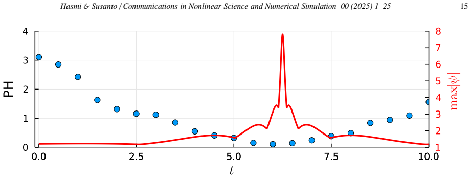
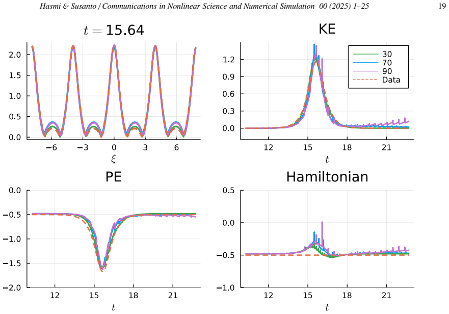
A properly tuned parallel Echo State Network, trained only on the quasi-periodic recurrence of an Ω ≈ 0.39799 breather with five unstable modes, predicts the one-step dynamics of three different datasets: the continuation of its own training trajectory, a fifth-order maximal intensity breather generated by a Darboux transformation, and random long-crested ocean waves drawn from a JONSWAP spectrum. One-step normalized errors stay small except near the instability peak, and autonomous forecasts give lead times of about two dimensionless time units ahead of a breather peak in the training continuation and around 0.5 time units for the maximal breather. The authors identify the obstacle for longer autonomous runs: the reservoir is intrinsically dissipative, so the predicted solution loses energy and drifts off the Hamiltonian flow; their remedy rescales the predicted field to conserve the initial norm and intermittently injects ground-truth data, which together capture both the amplitude and the timing of the rogue wave.
Load-bearing premise
The claim rests on one 70-time-unit training trajectory (after a 15-unit burn-in) adequately sampling the phase space of the NLS, including the unstable manifold around homoclinic orbits, so that the same reservoir generalizes without retraining to a maximal breather and to random seas.
Editorial extensions
If this is right
- Without any retraining, the same reservoir one-step-predicts wave fields whose spatial structure differs from its training data: a fifth-order maximal breather and JONSWAP random seas.
- Autonomous prediction already yields a lead time of roughly two dimensionless units before a breather peak in the continuation data, and about half a unit before the maximal breather peak.
- The norm-preserving and data-assimilation corrections, applied together, capture both amplitude and timing of a rogue wave that occurs about 5.64 time units after the forecast starts; applying either correction alone degrades one of the two.
- Training data that also includes random wave realizations (the RC_Cm model) broadens the sampled phase space and improves autonomous amplitude accuracy, even though the reservoir and input matrices are unchanged.
- The loss of the Hamiltonian property in autonomous mode is the dominant error source; energy diagnostics (kinetic, potential, and total Hamiltonian) track the divergence of the forecast.
Reading between the lines
- A practical deployment recipe follows implicitly: train the reservoir on cheap breather simulations, then use occasional buoy or gauge measurements as the assimilation updates—the norm rescaling needs no model at all.
- The phase-space-coverage requirement suggests an active sampling strategy: choose the training window adaptively by maximizing overlap with the unstable manifold, using the local stretching number as a guide, rather than taking an arbitrary 70-unit segment.
- The same combined correction likely transfers to other conservative wave models (e.g., modified NLS or the Davey-Stewartson system) wherever energy drift dominates the autonomous error.
- A sharper test of the generalization claim would be to train on a recurrence with different modulation parameters and test on the maximal breather of this paper; the one-step error near the peak should stay comparable if the mechanism is robust.
Editorial analysis
A structured set of objections, weighed in public.
Referee Report
Summary. The paper trains a parallel echo state network (RC_AB) on a focusing NLS simulation with five unstable modes and tests it on three types of data: a temporal continuation of the training trajectory, a fifth-order maximal intensity breather, and JONSWAP random sea states. Two prediction modes are considered: teacher-forced one-step prediction and autonomous (generative) prediction. The paper reports low one-step NRMSE on all test sets, modest autonomous prediction horizons (roughly 0.5-2 dimensionless time units), and proposes two corrections for autonomous mode: intermittent data assimilation (Section 6, Eq. (12)) and a per-step L2-norm rescaling (Eqs. (13)-(14)). The authors argue that the reservoir generalizes to unseen dynamics and that phase-space coverage of the training data is critical for Hamiltonian systems.
Significance. If the claims are fully supported, the paper would be a useful contribution to reservoir computing for Hamiltonian spatiotemporal systems, where attractor-based training arguments do not apply. The held-out random-realization test in Section 5 is a genuine strength, as is the explicit discussion of phase-space coverage in Section 7. The paper also gives credit for using translation-invariant parallel reservoirs and for attempting invariant-preserving corrections in autonomous mode. However, the central generalization claim is currently supported mainly by one-step NRMSE values that lack a persistence baseline, and the 'relatively long prediction horizon' is not quantified against any reference timescale. These gaps make the strongest form of the abstract's claim premature.
major comments (4)
- [Sections 2.3, 3.2, 4, 5 (Figs. 3, 8, 10)] The one-step prediction results are not benchmarked against a persistence baseline. With the reservoir sampling interval Δt_RC = 5×10^-3 (Section 3.2), the carrier phase of the NLS solution advances by only about 0.005 radians per step, and the fastest unstable mode (γ_max = 0.964) changes the envelope by roughly 0.5% per step. A persistence forecast ŷ_{j+1} = y_j, or the phase-rotated version ŷ_{j+1} = e^{iΔt_RC} y_j, would already produce very small NRMSE in smooth regions. Because the readout is trained to map the current state to its successor, low one-step error can reflect approximation of a near-identity map rather than learning of the NLS vector field or homoclinic structure. Please report NRMSE for these baselines alongside Figs. 3, 8, and 10, and discuss whether the RC one-step error is actually lower. The autonomous-mode figures are more discriminating and may survive, but the one-step evidence for 'unseen dynamics' is not conclusive without this baseline.
- [Abstract; Sections 3.3, 4, 5] The claim of a 'relatively long prediction horizon' is overstated relative to the reported results. Section 3.3 states that the RC can detect rogue waves approximately two time units before occurrence; Section 4 reports a lead time of 0.5 time units for the maximal intensity breather; Section 5 initiates autonomous prediction 0.13 dimensionless time units before the rogue wave event. Since γ_max^-1 ≈ 1.04 time units, the demonstrated horizons are of order one characteristic instability time, not clearly 'long' in any absolute sense. Please quantify the prediction horizon with explicit PH values at several starting times, compare against persistence-based autonomous prediction, and temper the abstract's 'relatively long prediction horizon' wording accordingly.
- [Sections 3.2 and 7] The conclusion that training data must sufficiently sample the phase space is explicitly stated in Section 7, but the paper does not provide evidence that the single 70-time-unit training trajectory from the Ω = 0.39799 breather simulation adequately spans the unstable manifold. This assumption is load-bearing for the generalization claims to the fifth-order maximal breather and to JONSWAP seas. Please support it with a concrete test, for example by training on multiple different time windows or multiple initial perturbations and showing that the prediction horizon and one-step errors are stable, or by measuring some proxy of phase-space coverage (e.g., local dimension or distribution of stretching numbers). Without such evidence, the phase-space coverage interpretation remains an untested hypothesis rather than a demonstrated mechanism.
- [Section 6, Eqs. (12)-(14), Figs. 12-13] The combined data-assimilation and norm-rescaling method is claimed to 'significantly extend the prediction horizon,' but no quantitative PH values are reported for the three scenarios (update only, normalization only, combined), and the method uses external ground-truth measurements at prescribed intervals. Please report the autonomous prediction horizon for each scenario and for several starting times t0, and clarify how much of the improvement is attributable to the intermittent injection of true data versus the norm rescaling. Note also that Eq. (14) imposes the initial L2 norm at every step by construction; this is a valid constraint for the NLS, whose L2 norm is conserved, but it is a hard constraint applied externally rather than a learned property, and it does not correct phase or timing errors, as Fig. 12 itself shows for the normalization-only case.
minor comments (5)
- [Section 2.3, Eq. (10)] In the definition of e_{j0,jl}, the ground-truth term in the numerator and denominator should be y_{j0+jl}, not y_j, to make the index conventions consistent with the preceding sentence.
- [Section 3.3 and Appendix B] The text says γ_max is 'equivalent to the largest Lyapunov exponent in the case of a plane wave solution,' while Appendix B states that the largest Lyapunov exponent is 'not well-defined' due to persistent fluctuations of the stretching number. Please reconcile these statements or clarify the distinction between the local stretching rate and a global Lyapunov exponent.
- [Section 5 and Appendix C] The time conversion in Eq. (C.1) uses the parameters T_p = 8 s and H_s = 8 m, but the paper does not state the value of the NLS scaling parameter ǫ used to set ||ψ|| = 1. Please specify this value, as it is needed to reproduce the reported physical times such as 1.32 s.
- [Data availability statement] The data availability statement says data are available in the article or supplementary materials, but no repository link, code, or detailed hyperparameter configuration file is provided. For reproducibility of the RC results, please make the training and testing datasets and the implementation available.
- [Throughout] There are several typos and formatting artifacts in the manuscript text, including 'Numerical Simulat ion' in the journal header and inconsistent spacing in equations; a careful proofread would improve presentation.
Circularity Check
No load-bearing circularity: the readout is fit to a held-out training segment and the main autonomous results are not forced by construction.
full rationale
The study is a supervised reservoir-computing experiment, not a derivation from first principles. The readout matrix Wo is the only trained parameter, obtained by ridge regression (Eqs. 6-8) on a 70-time-unit segment of one NLS breather simulation; the test sets (continuation, fifth-order maximal breather, JONSWAP realizations) are not used to solve for Wo. RC_Cm adds one random-wave realization to the training data but is evaluated on different realizations, so its assessment remains held out. The Section 6 corrections are explicitly external: data assimilation injects ground-truth states at sparse times (Eq. 12), and the norm rescaling (Eqs. 13-14) uses the L2 norm, which is a conserved quantity of the focusing NLS, not a learned parameter. No uniqueness theorem, self-citation chain, or renamed known result carries the argument. The paper even states the relevant limitation explicitly: 'the training data must sufficiently sample the phase space' (Section 7), conceding that generalization is conditional on phase-space coverage rather than guaranteed by construction. The one-step teacher-forcing results lack a persistence baseline, so low NRMSE may partly reflect the near-identity character of the map at dt_RC=5e-3, but this is a benchmarking gap, not circularity, because the reported errors are measured on unseen data and the autonomous predictions provide independent evidence.
Assumptions & free parameters
free parameters (11)
- Reservoir size per parallel RC (dS) =
800
- Number of parallel reservoirs (M) =
64
- Overlap length (l) =
4 (two physical nodes in real/imag parts)
- Input noise variance (sigma) =
0.02
- Tikhonov regularization (beta) =
1e-4
- Washout steps (Nw) =
100
- Sampling interval (Delta t_RC) =
0.005
- Spectral radius of reservoir matrix
- Input scaling (alpha)
- Partial update interval =
70 time steps (0.35 time units)
- NRMSE threshold (epsilon) =
0.4
assumptions (6)
- domain assumption The focusing nonlinear Schrödinger equation (Eq. 11) is an accurate model for rogue wave dynamics in deep water and optics.
- domain assumption The Clean Numerical Simulation with Taylor expansion and quadruple precision yields ground truth that represents true NLS dynamics, and truncation to double precision does not alter the conclusions.
- standard math The reservoir is assumed to have the echo state property, so hidden state dependence on initial conditions washes out after Nw washout steps.
- domain assumption A single shared output matrix Wo across all parallel reservoirs (translation invariance) is sufficient to capture the NLS dynamics on a uniform periodic grid.
- ad hoc to paper Rescaling the global L2 norm to its initial value at each step (Eq. 14) is a sufficient correction for the reservoir's dissipative energy drift.
- domain assumption The local maximum stretching number computed with piecewise-constant coefficients is a valid estimate of the local Lyapunov exponent for scaling prediction horizons.
Cite this review
Pith. "Pith review of Model-free Forecasting of Rogue Waves using Reservoir Computing." pith.science (2026). https://pith.science/paper/5GKPPMZC
@misc{pith2026250621918,
  author       = {Pith},
  title        = {Pith review of: Model-free Forecasting of Rogue Waves using Reservoir Computing},
  year         = {2026},
  howpublished = {\url{https://pith.science/paper/5GKPPMZC}},
  note         = {Machine review of arXiv:2506.21918}
}
read the original abstract
Recent research has demonstrated Reservoir Computing's capability to model various chaotic dynamical systems, yet its application to Hamiltonian systems remains relatively unexplored. This paper investigates the effectiveness of Reservoir Computing in capturing rogue wave dynamics from the nonlinear Schr\"{o}dinger equation, a challenging Hamiltonian system with modulation instability. The model-free approach learns from breather simulations with five unstable modes. A properly tuned parallel Echo State Network can predict dynamics from two distinct testing datasets. The first set is a continuation of the training data, whereas the second set involves a higher-order breather. An investigation of the one-step prediction capability shows remarkable agreement between the testing data and the models. Furthermore, we show that the trained reservoir can predict the propagation of rogue waves over a relatively long prediction horizon, despite facing unseen dynamics. Finally, we introduce a method to significantly improve the Reservoir Computing prediction in autonomous mode, enhancing its long-term forecasting ability. These results advance the application of Reservoir Computing to spatio-temporal Hamiltonian systems and highlight the critical importance of phase space coverage in the design of training data.
Figures


Figures from the paper (11 more)




Reference graph
Works this paper leans on
-
[1]
P . C. Liu, A chronology of freaque wave encounters, Geofiz ika 24 (1) (2007) 57 – 70. URL https://hrcak.srce.hr/file/2720
work page 2007
-
[2]
E. Didenkulova, Catalogue of rogue waves occurred in the World Ocean from 2011 to 2018 reported by mass media sources, Ocean and Coastal Management 188 (2020) 105076. doi:10.1016 /j.ocecoaman.2019.105076
arXiv 2020
- [3]
-
[4]
M. Christou, K. Ewans, Field Measurements of Rogue Water Waves, Journal of Physical Oceanography 44 (9) (2014) 2317– 2335. doi:10.1175/JPO-D-13-0199.1
- [5]
-
[6]
M. Onorato, A. R. Osborne, M. Serio, S. Bertone, Freak Wav es in Random Oceanic Sea States, Physical Review Letters 86 ( 25) (2001) 5831–5834. doi:10.1103 /PhysRevLett.86.5831
work page 2001
-
[7]
M. Onorato, A. R. Osborne, M. Serio, Modulational Instab ility in Crossing Sea States: A Possible Mechanism for the Fo rmation of Freak Waves, Physical Review Letters 96 (1) (2006) 014503. doi:10 .1103/PhysRevLett.96.014503
work page 2006
-
[8]
M. Onorato, D. Proment, A. To ffoli, Freak waves in crossing seas, The European Physical Jou rnal Special Topics 185 (1) (2010) 45–55. doi:10.1140/epjst/e2010-01237-8
Show all 70 references
-
[9]
Akhmediev, J
N. Akhmediev, J. M. Soto-Crespo, A. Ankiewicz, Extreme w aves that appear from nowhere: On the nature of rogue waves, P hysics Letters, Section A: General, Atomic and Solid State Physics 373 (25) ( 2009) 2137–2145. doi:10.1016 /j.physleta.2009.04.023
2009
-
[10]
W. M. Moslem, P . K. Shukla, B. Eliasson, Surface plasma r ogue waves, Europhysics Letters 96 (2) (2011) 25002. doi:10 .1209/0295- 5075/96/25002
2011
-
[11]
G. P . V eldes, J. Borhanian, M. McKerr, V . Saxena, D. J. Frantzeskakis, I. Kourakis, Electromagnetic rogue waves in beam–plasma interactions, Journal of Optics 15 (6) (2013) 064003. doi:10.1088 /2040-8978/15/6/064003
2013
-
[12]
Y ang, Y .-X
Y . Y ang, Y .-X. Gao, H.-W. Y ang, Analysis of the rogue waves in the blood based on the high-order NLS equations with var iable coefficients, Chinese Physics B 30 (11) (2021) 110202. doi:10.1088 /1674-1056/abff31
2021
-
[13]
Li, Z.-J
J. Li, Z.-J. Y ang, S.-M. Zhang, Characteristics of cert ain higher-order Hermite-cos-Gauss breathing solitons in duced by the initial wavefront bending in optical media with nonlocal nonlinearity, Chaos , Solitons & Fractals 187 (2024) 115338. doi:10.1016 /j.chaos.2024.115338
2024
-
[14]
Y . Liu, Z. Zhao, Rogue waves of the (2 + 1)-dimensional integrable reverse space–time nonlocal Sc hrödinger equation, Theoretical and Mathematical Physics 222 (1) (2025) 34–52. doi:10.1134 /S0040577925010040
2025
-
[15]
A. V . Slunyaev, D. E. Pelinovsky, E. N. Pelinovsky, Rogue waves in the sea: Observations, physics, and mathematics, Physics-Uspekhi 66 (2) (2023) 148–172. doi:10.3367 /UFNe.2021.08.039038. 23 Hasmi & Susanto / Communications in Nonlinear Science and Numerical Simulat ion 00 (...
2023
-
[16]
Klein, M
M. Klein, M. Dudek, G. F. Clauss, S. Ehlers, J. Behrendt, N. Hoffmann, M. Onorato, On the Deterministic Prediction of Water W aves, Fluids 5 (1) (2020) 9. doi:10.3390 /fluids5010009
2020
-
[17]
Cousins, M
W. Cousins, M. Onorato, A. Chabchoub, T. P . Sapsis, Pred icting ocean rogue waves from point measurements: An experi mental study for unidirectional waves, Physical Review E 99 (2019) 032201. d oi:10.1103/PhysRevE.99.032201
2019 doi
-
[18]
Farazmand, T
M. Farazmand, T. P . Sapsis, Reduced-order prediction o f rogue waves in two-dimensional deep-water waves, Journal of Computational Physics 340 (2017) 418–434. doi:10.1016 /j.jcp.2017.03.054
2017
-
[19]
Kagemoto, Forecasting a water-surface wave train wi th artificial intelligence- A case study, Ocean Engineering 207 (2020) 107380
H. Kagemoto, Forecasting a water-surface wave train wi th artificial intelligence- A case study, Ocean Engineering 207 (2020) 107380. doi:10.1016/j.oceaneng.2020.107380
2020
-
[20]
H. Kagemoto, Forecasting a water-surface wave train wi th artificial intelligence (Part 2) – Can the occurrence of fr eak waves be predicted with AI?, Ocean Engineering 252 (2022) 111205. doi:10.1016 /j.oceaneng.2022.111205
2022
-
[21]
Breunung, B
T. Breunung, B. Balachandran, Data-driven, high resol ution ocean wave forecasting and extreme wave predictions, Ocean Engineering 268 (2023) 113271. doi:10.1016 /j.oceaneng.2022.113271
2023
-
[22]
echo state
H. Jaeger, The "echo state" approach to analysing and tr aining recurrent neural networks – with an Erratum note, Tec h. rep., German National Research Center for Information Technology, (2001)
2001
-
[23]
Jaeger, H
H. Jaeger, H. Haas, Harnessing Nonlinearity: Predicti ng Chaotic Systems and Saving Energy in Wireless Communication, Science 304 (5667) (2004) 78–80. doi:10.1126 /science.1091277
2004
-
[24]
Lukoševi ˇcius, H
M. Lukoševi ˇcius, H. Jaeger, Reservoir computing approaches to recurre nt neural network training, Computer Science Review 3 (3) (2 009) 127–149. doi:10.1016 /j.cosrev.2009.03.005
2009
-
[25]
Chattopadhyay, P
A. Chattopadhyay, P . Hassanzadeh, D. Subramanian, Data-driven predictions of a multiscale Lorenz 96 chaotic system using machine-learning methods: Reservoir computing, artificial neural network, a nd long short-term memory network, Nonlinear Processes in G eophysics 27 (3) (20...
2020
-
[26]
Pathak, Z
J. Pathak, Z. Lu, B. R. Hunt, M. Girvan, E. Ott, Using mach ine learning to replicate chaotic attractors and calculate Lyapunov exponents from data, Chaos: An Interdisciplinary Journal of Nonlinea r Science 27 (12) (2017) 121102, publisher: American Instit ute of Physics. doi:...
2017 doi
-
[27]
Pathak, B
J. Pathak, B. Hunt, M. Girvan, Z. Lu, E. Ott, Model-Free P rediction of Large Spatiotemporally Chaotic Systems from D ata: A Reservoir Computing Approach, Physical Review Letters 120 (2) (2018) 24102. doi:10.1103 /PhysRevLett.120.024102
2018
-
[28]
N. A. Doan, W. Polifke, L. Magri, Short- And long-term pr edictions of chaotic flows and extreme events: A physics-con strained reser- voir computing approach, Proceedings of the Royal Society A : Mathematical, Physical and Engineering Sciences 477 (202 1) 2253. doi:10.1098/rsp...
-
[29]
A. Röhm, D. J. Gauthier, I. Fischer, Model-free inferen ce of unseen attractors: Reconstructing phase space featur es from a single noisy trajectory using reservoir computing, Chaos 31 (2021) 1031 27. doi:10.1063 /5.0065813
2021
-
[30]
D. J. Gauthier, I. Fischer, A. Röhm, Learning unseen coe xisting attractors, Chaos: An Interdisciplinary Journal o f Nonlinear Science 32 (11) (2022) 113107, publisher: American Institute of Physics. d oi:10.1063/5.0116784
2022 doi
-
[31]
F. Huhn, L. Magri, Gradient-free optimization of chaot ic acoustics with reservoir computing, Physical Review Flu ids 7 (2022) 014402. doi:10.1103/PhysRevFluids.7.014402
2022 doi
-
[32]
Jiang, Y
J. Jiang, Y . C. Lai, Model-free prediction of spatiotem poral dynamical systems with recurrent neural networks: Ro le of network spectral radius, Physical Review Research 1 (2019) 033056. doi:10.1 103/PhysRevResearch.1.033056
2019
-
[33]
Pandey, J
S. Pandey, J. Schumacher, Reservoir computing model of two-dimensional turbulent convection, Physical Review Fl uids 5 (11) (2020) 113506. doi:10.1103 /PhysRevFluids.5.113506
2020
-
[34]
K. Y ao, E. Forgoston, P . Y ecko, Learning ocean circulat ion models with reservoir computing, Physics of Fluids 34 (1 1) (2022) 116604. doi:10.1063/5.0119061
2022 doi
-
[35]
Bonas, C
M. Bonas, C. K. Wikle, S. Castruccio, Calibrated foreca sts of quasi-periodic climate processes with deep echo stat e networks and penalized quantile regression, Environmetrics 35 (1) (2024) e2833. d oi:10.1002/env.2833. URL https://onlinelibrary.wiley.com/doi/abs/10.1002/env.2833
2024 doi
-
[36]
Pathak, A
J. Pathak, A. Wikner, R. Fussell, S. Chandra, B. R. Hunt, M. Girvan, E. Ott, Hybrid forecasting of chaotic processes: Using machine learning in conjunction with a knowledge-based model, Chaos: An Inte rdisciplinary Journal of Nonlinear Science 28 (4) (2018) 04 1101, publisher:...
2018
-
[37]
Wikner, J
A. Wikner, J. Pathak, B. Hunt, M. Girvan, T. Arcomano, I. Szunyogh, A. Pomerance, E. Ott, Combining machine learning with knowledge- based modeling for scalable forecasting and subgrid-scale closure of large, complex, spatiotemporal systems, Chaos 3 0 (5) (2020) 053111. doi:10...
2020 doi
-
[38]
Tanaka, T
G. Tanaka, T. Y amane, J. B. Héroux, R. Nakane, N. Kanazaw a, S. Takeda, H. Numata, D. Nakano, A. Hirose, Recent advance s in physical reservoir computing: A review, Neural Networks 115 (2019) 1 00–123. arXiv:1808.04962, doi:10.1016 /j.neunet.2019.03.005
2019 arXiv
-
[39]
Liang, J
X. Liang, J. Tang, Y . Zhong, B. Gao, H. Qian, H. Wu, Physic al reservoir computing with emerging electronics, Nature E lectronics 7 (3) (2024) 193–206. doi:10.1038 /s41928-024-01133-z
2024
-
[40]
Everschor-Sitte, A
K. Everschor-Sitte, A. Majumdar, K. Wolk, D. Meier, Top ological magnetic and ferroelectric systems for reservoir computing, Nature Re- views Physics 6 (7) (2024) 455–462. doi:10.1038 /s42254-024-00729-w
2024
-
[41]
Zhang, H
H. Zhang, H. Fan, L. Wang, X. Wang, Learning Hamiltonian dynamics with reservoir computing, Physical Review E 104 (2 ) (2021) 024205. doi:10.1103/PhysRevE.104.024205
2021 doi
-
[42]
Pershin, C
A. Pershin, C. Beaume, K. Li, S. M. Tobias, Training a neu ral network to predict dynamics it has never seen, Physical R eview E 107 (1) (2023) 014304. doi:10.1103 /PhysRevE.107.014304
2023
-
[43]
J. Z. Kim, Z. Lu, E. Nozari, G. J. Pappas, D. S. Bassett, Te aching recurrent neural networks to infer global temporal s tructure from local examples, Nature Machine Intelligence 3 (4) (2021) 316–323 . doi:10.1038 /s42256-021-00321-2
2021
-
[44]
Manjunath, H
G. Manjunath, H. Jaeger, Echo State Property Linked to a n Input: Exploring a Fundamental Characteristic of Recurre nt Neural Networks, Neural Computation 25 (3) (2013) 671–696. doi:10.1162 /NECO_a_0411
2013
-
[45]
W. A. Barbosa, A. Gri ffith, G. E. Rowlands, L. C. Govia, G. J. Ribeill, M. H. Nguyen, T. A. Ohki, D. J. Gauthier, Symmetry-aware reservoir 24 Hasmi & Susanto / Communications in Nonlinear Science and Numerical Simulat ion 00 (2025) 1–25 25 computing, Physical Review E 104 (2021...
2025
-
[46]
R. Pyle, N. Jovanovic, D. Subramanian, K. V . Palem, A. B. Patel, Domain-driven models yield better predictions at lo wer cost than reser- voir computers in Lorenz systems, Philosophical Transacti ons of the Royal Society A: Mathematical, Physical and Engin eering Sciences 379...
2021
-
[47]
N. N. Akhmediev, V . M. Eleonskii, N. E. Kulagin, Exact fir st-order solutions of the nonlinear Schrödinger equation, Theoretical and Mathe- matical Physics 72 (2) (1987) 809–818. doi:10.1007 /BF01017105
1987
-
[48]
B. M. Herbst, M. J. Ablowitz, Numerically induced chaos in the nonlinear schrödinger equation, Physical Review Let ters 62 (18) (1989) 2065–2068. doi:10.1103 /PhysRevLett.62.2065
1989
-
[49]
M. R. Beli ´c, S. N. Nikoli ´c, O. A. Ashour, N. B. Aleksi ´c, On di fferent aspects of the optical rogue waves nature, Nonlinear D ynamics 108 (2) (2022) 1655–1670. doi:10.1007 /s11071-022-07284-y
2022
-
[50]
T. Hu, S. Liao, On the risks of using double precision in n umerical simulations of spatio-temporal chaos, Journal of Computational Physics 418 (2020) 109629. doi:10.1016 /j.jcp.2020.109629
2020
-
[51]
H. C. Y uen, W. E. Ferguson, Relationship between Benjam in-Feir instability and recurrence in the nonlinear Schröd inger equation, Physics of Fluids 21 (8) (1978) 1275–1278. doi:10.1063 /1.862394
1978
-
[52]
Erkintalo, K
M. Erkintalo, K. Hammani, B. Kibler, C. Finot, N. Akhmed iev, J. M. Dudley, G. Genty, Higher-order modulation instability in nonlinear fiber optics, Physical Review Letters 107 (25) (2011) 14–18. doi: 10.1103/PhysRevLett.107.253901
2011 doi
-
[53]
S. A. Chin, O. A. Ashour, M. R. Beli ´c, Anatomy of the Akhmediev breather: Cascading instability, first formation time, and Fermi-Pasta-Ulam recurrence, Physical Review E 92 (6) (2015) 063202. doi:10. 1103/PhysRevE.92.063202
2015
-
[54]
M. Roy, S. Mandal, C. Hens, A. Prasad, N. V . Kuznetsov, M. Dev Shrimali, Model-free prediction of multistability usi ng echo state network, Chaos: An Interdisciplinary Journal of Nonlinear Science 3 2 (10) (2022) 101104. doi:10.1063 /5.0119963
2022
-
[55]
S. A. Chin, O. A. Ashour, S. N. Nikoli ´c, M. R. Beli ´c, Maximal intensity higher-order Akhmediev breathers of t he nonlinear Schrödinger equation and their systematic generation, Physics Letters , Section A: General, Atomic and Solid State Physics 380 (43) (2016) 3625–3629. ...
2016 doi
-
[56]
Akhmediev, N
N. Akhmediev, N. Mitzkevich, Extremely high degree of N -soliton pulse compression in an optical fiber, IEEE Journal of Quantum Electronics 27 (3) (1991) 849–857. doi:10.1109 /3.81399
1991
-
[57]
D. J. Kedziora, A. Ankiewicz, N. Akhmediev, Circular ro gue wave clusters, Physical Review E - Statistical, Nonline ar, and Soft Matter Physics 84 (5) (2011) 056611. doi:10.1103 /PhysRevE.84.056611
2011
-
[58]
H. Fan, J. Jiang, C. Zhang, X. Wang, Y . C. Lai, Long-term p rediction of chaotic systems with machine learning, Physic al Review Research 2 (1) (2020) 012080. doi:10.1103 /PhysRevResearch.2.012080
2020
-
[59]
T. P . Sapsis, Statistics of Extreme Events in Fluid Flow s and Waves, Annual Review of Fluid Mechanics 53 (2021) 85–11 1. doi:10.1146/annurev-fluid-030420-032810
2021 doi
-
[60]
Fujii, K
K. Fujii, K. Nakajima, Harnessing Disordered-Ensembl e Quantum Dynamics for Machine Learning, Physical Review Ap plied 8 (2) (2017) 024030. doi:10.1103 /PhysRevApplied.8.024030
2017
-
[61]
W. A. S. Barbosa, D. J. Gauthier, Learning spatiotempor al chaos using next-generation reservoir computing, Chaos : An Interdisciplinary Journal of Nonlinear Science 32 (9) (2022) 093137, publishe r: American Institute of Physics. doi:10.1063 /5.0098707
2022
-
[62]
P . J. Ehlers, H. I. Nurdin, D. Soh, Stochastic reservoir computers, Nature Communications 16 (1) (2025) 3070. doi:1 0.1038/s41467-025- 58349-6
2025
- [63]
-
[64]
V oglis, G
N. V oglis, G. J. Contopoulos, Invariant spectra of orbi ts in dynamical systems, Journal of Physics A: Mathematical and General 27 (14) (1994) 4899. doi:10.1088 /0305-4470/27/14/017
1994
-
[65]
Eckhardt, D
B. Eckhardt, D. Y ao, Local Lyapunov exponents in chaoti c systems, Physica D: Nonlinear Phenomena 65 (1) (1993) 100– 108. doi:10.1016/0167-2789(93)90007-N
1993 doi
-
[66]
Skokos, E
C. Skokos, E. Gerlach, Numerical integration of variat ional equations, Physical Review E 82 (3) (2010) 036704. doi:10.1103/PhysRevE.82.036704
2010 doi
-
[67]
Skokos, The Lyapunov Characteristic Exponents and T heir Computation, in: Dynamics of Small Solar System Bodies and Exoplanets, Springer, Berlin, Heidelberg, 2010, pp
C. Skokos, The Lyapunov Characteristic Exponents and T heir Computation, in: Dynamics of Small Solar System Bodies and Exoplanets, Springer, Berlin, Heidelberg, 2010, pp. 63–135. doi:10.10 07/978-3-642-04458-8_2
2010
-
[68]
Kharif, E
C. Kharif, E. Pelinovsky, A. Slunyaev, Rogue Waves in th e Ocean, Advances in Geophysical and Environmental Mechanics and Mathematics, Springer, Berlin, Heidelberg, 2009. doi:10.1007 /978-3-540-88419-4
2009
-
[69]
Hasselmann, T
K. Hasselmann, T. Barnett, E. Bouws, H. Carlson, D. Cart wright, K. Enke, J. Ewing, H. Gienapp, D. Hasselmann, P . Kruseman, A. Meerburg, P . Muller, D. Olbers, K. Richter, W. Sell, H. Walden, Measure ments of wind-wave growth and swell decay during the joint no rth sea wave p...
1973
-
[70]
Mackay, A unified model for unimodal and bimodal ocean wave spectra, International Journal of Marine Energy 15 (20 16) 17–40
E. Mackay, A unified model for unimodal and bimodal ocean wave spectra, International Journal of Marine Energy 15 (20 16) 17–40. doi:10.1016/j.ijome.2016.04.015. 25
2016 doi
Reviewed August 6, 2026 · model on record in the stance chip above.
Discussion (0). Continue with ORCID to comment.