REVIEW 2 major objections 5 minor 24 references
Pricing and Calibration of VIX Derivatives in Mixed Bergomi Models via Quantisation
T0 review · 2 major / 5 minor · reviewed 2026-08-06 · deepseek-v4-flash
Pith's one-line read Vector quantisation makes daily VIX Bergomi calibration feasible.
desk verdict Solid quantisation speed-up for Bergomi VIX pricing, but the corridor-only calibration objective leaves parameters unidentified, so the stability claims need to be reframed. read the letter →
The pith
A machine-rendered reading of the paper's core claim, the machinery that carries it, and where it could break.
The reading
What carries the argument
The load-bearing object is the $L^2$-optimal $N$-point Gaussian quantiser: a fixed grid $\{y_1,\ldots,y_N\}$ with Voronoi probabilities $p_j$ that replaces a continuous Gaussian random variable by a discrete proxy. In the one-factor model, the Ornstein-Uhlenbeck state $X_t$ is scaled from a 1,000-point univariate normal quantiser; in the two-factor model, a 1,450-point bivariate normal quantiser is transformed by Cholesky decomposition to match the correlation of the two OU drivers. Because $V IX^2_{T_i}$ is a deterministic function of the quantised state, the VIX futures price becomes $\sum_j \sqrt{V^j_i}\,p_j$ and call/put prices become analogous sums of payoffs, with a 20-node Gauss-Legendre rule handling the time integral. These precomputed grids and simple weighted sums, rather than multi-dimensional numerical integration, are what deliver the speed.
What would settle it
Take one daily maturity slice and rerun the same calibration from many random starting parameter vectors, recording the final objective value and the returned $(\gamma_T, \omega_T^1, \omega_T^2)$. If the objective remains at the same near-zero level while the parameters scatter widely within the bid-ask corridor, the point estimates and their time-series stability are not identified, independent of how fast quantisation makes the pricing.
Extended reading notes
Core claim
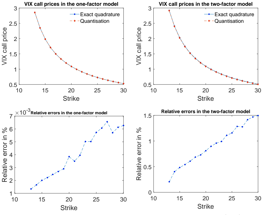
The central claim is that vector quantisation can replace exact quadrature as the pricing engine for mixed Bergomi models without sacrificing accuracy. Using a 1,000-point univariate normal grid for the one-factor model and a 1,450-point bivariate normal grid for the two-factor model, the authors compute VIX futures, calls, and puts as weighted sums over the grid; the resulting prices agree with exact quadrature to within $0.001\%$, $0.007\%$, and $0.00035\%$ (one-factor) and $0.1\%$, $1.5\%$, and $0.4\%$ (two-factor) for futures, calls, and puts, respectively, while running twice as fast in the one-factor model and about 120 times as fast in the two-factor model. On this basis the paper jointly calibrates the models, maturity slice by maturity slice, to 105 daily VIX futures and call surfaces with maturities from one week to nine months. The calibration errors are tiny—mean relative futures errors around $3.5\times 10^{-5}$ and mean relative bid-ask errors for calls around $3\times 10^{-5}$—and the calibrated parameters show reasonable, though not perfect, stability over time.
Load-bearing premise
The calibration objective in Section 4.2 penalises only model call prices that fall outside the bid-ask corridor, so the reported point estimates of $\gamma_T$, $\omega_T^1$, and $\omega_T^2$ are not uniquely identified from the data; the apparent stability of the parameter paths could be an artifact of the optimizer's arbitrary choice inside that flat region.
Editorial extensions
If this is right
- Daily recalibration of mixed one- and two-factor Bergomi models to VIX derivatives becomes practical, because quantisation is about twice as fast as exact quadrature in the one-factor model and about 120 times faster in the two-factor model.
- Both models fit the observed VIX futures and call surfaces almost perfectly in single-day cross-sectional calibration, with mean relative errors on the order of $10^{-5}$.
- If the objective is only to calibrate VIX futures and options, the mixed one-factor Bergomi model is sufficient; the two-factor model's extra factor buys only a marginal improvement.
- The term structure of initial forward variance $\xi_0^T$ is the dominant driver of pricing accuracy, so refreshing $\xi_0^T$ daily while keeping the other parameters fixed preserves most of the fit to VIX futures.
- When calibrated parameters are held fixed, out-of-sample pricing errors stabilise after about six days rather than growing, suggesting the models capture VIX derivative dynamics over at least a month.
Reading between the lines
- The paper leaves implicit that the reported parameter stability is conditional on the flat bid-ask corridor objective; a strictly convex penalty term would be needed to identify $\gamma_T$, $\omega_T^1$, and $\omega_T^2$ uniquely.
- Because the Gaussian quantiser grids are precomputed once and reused, the speed advantage should carry over to real-time pricing, risk management, and scenario simulation for VIX derivatives, not just calibration.
- A natural extension would be to apply the same grid-quantisation machinery to other Markovian forward-variance models, or to use adaptive or recursive quantisation to refine the grid in regions that matter for deep out-of-the-money strikes.
- The dominance of $\xi_0^T$ suggests a practical workflow: strip the forward variance term structure from VIX futures daily, and recalibrate the smile parameters on a slower cadence such as weekly.
Signed reviews
Editorial analysis
A structured set of objections, weighed in public.
Referee Report
Summary. The paper applies vector quantisation (precomputed optimal Gaussian grids) to price VIX futures and options in mixed one- and two-factor Bergomi models. It benchmarks quantisation against exact quadrature, reports speedups, and then calibrates the per-maturity parameters (γ_T, ω_T^1, ω_T^2, ξ_0^T) slice-by-slice to 105 days of CBOE VIX futures and call data using a corridor-type loss. It evaluates static fit and parameter stability, including four fixed-parameter out-of-sample tests. The authors conclude that both models fit VIX derivatives with near-perfect in-sample accuracy and satisfactory parameter stability, and that ξ_0^T is the dominant driver of pricing accuracy.
Significance. If the numerical claims are correct, the paper offers a practical speedup for recalibrating mixed Bergomi models to VIX derivatives: the accuracy tests are benchmarked against exact quadrature with small relative errors, and the calibration over 1,213 maturity slices is a useful empirical exercise. The proposed one-step parametrisation of the two-factor model is also convenient. The paper is honest about the static-vs-dynamic distinction and provides several out-of-sample tests with fixed parameters, which is a strength. The main weakness is that the corridor-only objective leaves per-slice parameters unidentified, so the stability assessment is not as solid as the pricing methodology. The paper also provides MATLAB code for the accuracy tests, which supports reproducibility of the numerical claims.
major comments (2)
- [Section 4.2, objective function] The call-option term is a sum of squared positive deviations outside the bid-ask corridor, so it vanishes identically whenever all model call prices fall inside the corridor. With four free parameters per slice (γ_T, ω_T^1, ω_T^2, ξ_0^T) and only the single VIX futures equation active on that region, the minimizer is generically non-unique; fmincon then returns a point determined by starting values and algorithm details. Consequently, the daily parameter paths in Section 5.1 (Figures 9-12) and the Abstract/Conclusion statements about 'satisfactory stability' describe an arbitrary selection within the flat region rather than identified model parameters. This does not affect the quantisation speed/accuracy claim, but it is load-bearing for the dynamic-stability assessment. Please remedy by reporting corridor widths and multi-start dispersion, using a mid-price or penalty-anchored objective, or substantially qualifying the stability claims.
- [Equations (12)-(14) and Tables 2-4] The reported ARBAE and RBAE measure only violations outside the bid-ask corridor, not deviations from mid-market prices. Near-zero values therefore mean that model prices lie within the bid-ask bounds, which is weaker than 'near-perfect fits' to market prices. Since the Conclusion states that both models achieve near-perfect fits to VIX futures and calls, the corridor-only metrics overstate static performance. Please supplement with mid-price errors, such as root mean squared relative error against mid quotes, or at least report the fraction of quotes priced inside the corridor.
minor comments (5)
- [Figure 8] The vertical axis label '9T0' appears to be a rendering error; it should read ξ_0^T.
- [Section 3.1] The word 'calender' is a typo and should be 'calendar'.
- [Section 1] The phrase 'In the literature:' contains a stray colon and should be 'In the literature,'.
- [Reference [16]] The reference is listed as 'Eduardo Abi Jaber et al.' without full author details; please complete the bibliographic entry.
- [Section 3.4] To make the 2x and 120x speedups reproducible, please report the hardware, MATLAB version, quadrature tolerance settings, and number of timing repetitions.
Circularity Check
No significant circularity: the pricing benchmark is independent exact quadrature, and the stability claims rest on out-of-sample fixed-parameter tests.
full rationale
The paper's derivation chain is self-contained. Quantisation accuracy is assessed against exact quadrature, which is an external numerical benchmark independent of the calibrated parameters, and the reported speed gains are direct computational measurements rather than consequences of the model equations. The in-sample calibration fit is explicitly presented as calibration accuracy, not as an out-of-sample prediction, so using the same relative-error metrics in the objective and in the summary statistics is standard fitting behaviour rather than a reduction by construction. The parameter-stability claims are supported by Tests 1 to 4, which fix the calibrated parameters for up to 30 trading days and price subsequent daily surfaces, with only the initial forward variance refreshed either by the model-independent replication formula (15) or by recalibration; this is genuine out-of-sample pricing relative to the fitted parameters. The use of equation (15) to strip the initial forward variance from VIX futures and options is a market-data input, and the model futures price is then computed from the full distribution of VIX, so the futures match is not forced by construction. The self-citations to Bergomi's mixed-model constructions and to similar objective functions in the literature are background modelling choices, not load-bearing justifications that import the paper's conclusions. The flatness of the calibration objective inside the bid-ask corridor noted in the reader's take is an identifiability concern about non-unique optima, not a circularity: it does not make any derived quantity equivalent to its own input. No equation in the paper is defined in terms of the quantity it is used to predict, and no fitted parameter is renamed as an independent prediction.
Assumptions & free parameters
free parameters (6)
- gamma_T (mixing weight, one- and two-factor) =
e.g. 0.9154 for one-factor, T=7 days, 09 Apr 2024; varies by slice and day
- omega_T^1 (vol-of-vol, first component) =
e.g. 17.98 for one-factor, T=7 days, 09 Apr 2024
- omega_T^2 (vol-of-vol, second component) =
e.g. 1.28 for one-factor, T=7 days, 09 Apr 2024
- xi_0^T (initial forward variance) =
e.g. 0.0234 for one-factor, T=7 days, 09 Apr 2024; also stripped from market via Eq. (15)
- k (one-factor mean reversion) =
1
- k1, k2, theta, rho (two-factor structure) =
7.54, 0.24, 0.23, 0.7 (Set III from Bergomi)
assumptions (5)
- domain assumption The forward variance curve xi_t^T is a martingale in t under the risk-neutral measure Q.
- domain assumption VIX squared is the integral of forward variances over the next 30 days, VIX_t^2 = (100^2 / Delta) * integral from t to t+Delta of xi_t^T dT.
- domain assumption The optimal quantisers for standard normal and bivariate normal distributions downloaded from the Quantisation Website are accurate enough for pricing.
- domain assumption Parameters gamma_T, omega_T^1, omega_T^2, and xi_0^T are constant on the interval [T_i, T_i + Delta] for each calibration slice.
- domain assumption Market option prices satisfy put-call parity, so the risk-free rate r and futures price F can be extracted by least squares.
Cite this review
Pith. "Pith review of Pricing and Calibration of VIX Derivatives in Mixed Bergomi Models via Quantisation." pith.science (2026). https://pith.science/paper/OGLN7HSU
@misc{pith2026250623409,
  author       = {Pith},
  title        = {Pith review of: Pricing and Calibration of VIX Derivatives in Mixed Bergomi Models via Quantisation},
  year         = {2026},
  howpublished = {\url{https://pith.science/paper/OGLN7HSU}},
  note         = {Machine review of arXiv:2506.23409}
}
read the original abstract
We apply vector quantisation within mixed one- and two-factor Bergomi models to implement a fast and efficient approach for option pricing in these models. This allows us to calibrate such models to market data of VIX futures and options. Our numerical tests confirm the efficacy of vector quantisation, making calibration feasible over daily data covering several months. This permits us to evaluate the calibration accuracy and the stability of the calibrated parameters, and we provide a comprehensive assessment of the two models. Both models show excellent performance in fitting VIX derivatives, and their parameters show satisfactory stability over time.
Figures


Figures from the paper (11 more)


Reference graph
Works this paper leans on
-
[1]
http://www.quantize.maths-fi.com/gaussian_database, [Online; accessed April 2024]
QuantizationWebsite. http://www.quantize.maths-fi.com/gaussian_database, [Online; accessed April 2024]
work page 2024
-
[2]
Eduardo Abi Jaber, Camille Illand, and Shaun Li. Joint SPX & VIX calibration with Gaussian polynomial volatility models: Deep pricing with quantization hints. Mathematical Finance, 2022
work page 2022
-
[3]
A consistent stochastic model of the term structure of interest rates for multiple tenors
Mesias Alfeus, Martino Grasselli, and Erik Schlögl. A consistent stochastic model of the term structure of interest rates for multiple tenors. Journal of Economic Dynamics and Control, 114:103861, 2020
work page 2020
-
[4]
Smile dynamics II.Risk, pages 67–73, October 2005
Lorenzo Bergomi. Smile dynamics II.Risk, pages 67–73, October 2005
work page 2005
-
[5]
Smile dynamics III.Risk, pages 90–96, October 2008
Lorenzo Bergomi. Smile dynamics III.Risk, pages 90–96, October 2008
work page 2008
-
[6]
Stochastic volatility modeling
Lorenzo Bergomi. Stochastic volatility modeling. CRC press, 2015
work page 2015
-
[7]
Florian Bourgey, Stefano De Marco, and Emmanuel Gobet. Weak approximations and VIX option price expansions in forward variance curve models.Quantitative Finance, 23(9):1259–1283, 2023
work page 2023
-
[8]
Giorgia Callegaro, Lucio Fiorin, and Martino Grasselli. Pricing and calibration in local volatility models via fast quantization.Available at SSRN 2495829, 2014
work page 2014
Show all 24 references
-
[9]
Pricing via recursive quan- tization in stochastic volatility models.Quantitative Finance, 17(6):855–872, 2017
Giorgia Callegaro, Lucio Fiorin, and Martino Grasselli. Pricing via recursive quan- tization in stochastic volatility models.Quantitative Finance, 17(6):855–872, 2017
2017
-
[10]
Towards a theory of volatility trading.Option Pric- ing, Interest Rates and Risk Management, Handbooks in Mathematical Finance, 22(7):458–476, 2001
Peter Carr and Dilip Madan. Towards a theory of volatility trading.Option Pric- ing, Interest Rates and Risk Management, Handbooks in Mathematical Finance, 22(7):458–476, 2001
2001
-
[11]
Theinformation contentoftheS&P500indexandVIXoptionsonthedynamicsoftheS&P500index
San-LinChung, Wei-CheTsai, Yaw-HueiWang, andPei-ShihWeng. Theinformation contentoftheS&P500indexandVIXoptionsonthedynamicsoftheS&P500index. Journal of Futures Markets, 31(12):1170–1201, 2011
2011
-
[12]
Joint cal- ibration to SPX and VIX options with signature-based models.Mathematical Fi- nance, 2023
Christa Cuchiero, Guido Gazzani, Janka Möller, and Sara Svaluto-Ferro. Joint cal- ibration to SPX and VIX options with signature-based models.Mathematical Fi- nance, 2023
2023
-
[13]
The VIX future in Bergomi models: Fast approximation formulas and joint calibration with S&P 500 skew.SIAM Journal on Financial Mathematics, 13(4):1418–1485, 2022
Julien Guyon. The VIX future in Bergomi models: Fast approximation formulas and joint calibration with S&P 500 skew.SIAM Journal on Financial Mathematics, 13(4):1418–1485, 2022. 27
2022
-
[14]
Dispersion-constrainedmartingaleschrödingerproblemsandtheexact joint S&P 500/VIX smile calibration puzzle.Finance and Stochastics, 28(1):27–79, 2024
JulienGuyon. Dispersion-constrainedmartingaleschrödingerproblemsandtheexact joint S&P 500/VIX smile calibration puzzle.Finance and Stochastics, 28(1):27–79, 2024
2024
-
[15]
Does the term-structure of equity at-the-money skew really follow a power law?Risk, pages 1–6, August 2023
Julien Guyon and Mehdi El Amrani. Does the term-structure of equity at-the-money skew really follow a power law?Risk, pages 1–6, August 2023
2023
-
[16]
Volatility models in practice: Rough, Path-dependent or Markovian? arXiv preprint arXiv:2401.03345, 2024
Eduardo Abi Jaber et al. Volatility models in practice: Rough, Path-dependent or Markovian? arXiv preprint arXiv:2401.03345, 2024
2024 arXiv
-
[17]
The quintic Ornstein-Uhlenbeck volatility model that jointly calibrates SPX & VIX smiles.Risk, pages 1–6, July 2023
Eduardo Abi Jaber, Camille Illand, et al. The quintic Ornstein-Uhlenbeck volatility model that jointly calibrates SPX & VIX smiles.Risk, pages 1–6, July 2023
2023
-
[18]
Joint pricing of VIX and SPX options with stochastic volatility and jump models
Thomas Kokholm and Martin Stisen. Joint pricing of VIX and SPX options with stochastic volatility and jump models. The Journal of Risk Finance, 16(1):27–48, 2015
2015
-
[19]
Callegaro O
G. Callegaro O. Bonesini and A. Jacquier. Functional quantization of rough volatility and applications to volatility derivatives.Quantitative Finance, 23(12):1769–1792, 2023
2023
-
[20]
Forward variance dynamics: Bergomi’s model revisited
Sidi Mohamed Ould Aly. Forward variance dynamics: Bergomi’s model revisited. Applied Mathematical Finance, 21(1):84–107, 2014
2014
-
[21]
Optimal quadratic quantization for numerics: the Gaussian case.Monte Carlo Methods Appl., 9(2):135–165, 2003
Gilles Pagès and Jacques Printems. Optimal quadratic quantization for numerics: the Gaussian case.Monte Carlo Methods Appl., 9(2):135–165, 2003
2003
-
[22]
Recursive marginal quantization of the Euler scheme of a diffusion process.Applied Mathematical Finance, 22(5):463–498, 2015
Gilles Pagès and Abass Sagna. Recursive marginal quantization of the Euler scheme of a diffusion process.Applied Mathematical Finance, 22(5):463–498, 2015
2015
-
[23]
Empirical analysis of rough and classical stochastic volatility models to the SPX and VIX markets.Quantitative Finance, 22(10):1805–1838, 2022
Sigurd Emil Rømer. Empirical analysis of rough and classical stochastic volatility models to the SPX and VIX markets.Quantitative Finance, 22(10):1805–1838, 2022
2022
-
[24]
Legendre-Gauss quadrature weights and nodes.Matlab function lgwt
Greg Von Winckel. Legendre-Gauss quadrature weights and nodes.Matlab function lgwt. URL: http://www. mathworks. com/matlabcentral/fileexchange/4540 Wessel P, Smith WHF (1998), New, improved version of the Generic Mapping Tools released, EOS Trans. AGU, 79:579, 2004. 28
1998
Reviewed August 6, 2026 · model on record in the stance chip above.
Discussion (0). Continue with ORCID to comment.