ViscoReg: Neural Signed Distance Functions via Viscosity Solutions

Meenakshi Krishnan; Ramani Duraiswami

REVIEW 4 major objections 6 minor 18 references

ViscoReg: Neural Signed Distance Functions via Viscosity Solutions

T0 review · 4 major / 6 minor · reviewed 2026-08-06 · deepseek-v4-flash

Challenge this review Re-run · record.json Download PDF Read on arXiv ↗

Pith's one-line read The paper claims that adding a decaying viscosity term to the Eikonal loss stabilizes Neural SDF training and proves a generalization bound in which finite-sample training error controls worst-case error against the true SDF.

desk verdict ViscoReg the regularizer looks empirically useful, but the 'provably stabilizes' claim rests on a linearization that does not hold, and the generalization bound has a gap; worth a serious referee but needs real repair. read the letter →

arxiv 2507.00412 v2 pith:ZKY4OIIF submitted 2025-07-01 cs.GR

Meenakshi Krishnan , Ramani Duraiswami This is my paper

classification cs.GR MSC 35D4035F2168T07

keywords neuralsigneddistancefunctionsviscositysolutionsEikonalequationimplicitrepresentationssurfacereconstructiongeneralizationerrorvanishingpointclouds

verification ladder T0 review T1 audit T2 compute T3 formal

The pith

A machine-rendered reading of the paper's core claim, the machinery that carries it, and where it could break.

The reading

Neural networks that represent 3D surfaces as signed distance functions are typically trained by penalizing violations of the Eikonal equation, but that equation has infinitely many solutions and its gradient flow is unstable in practice. This paper argues that both troubles are cured by viscosity solution theory, the classical framework that selects the true signed distance function as the unique viscosity solution of the Eikonal equation. The paper proves a generalization bound (Theorem 1): for the trained network, the worst-case (infinity-norm) error against the ground-truth SDF is at most a constant times the square roots of the boundary and Eikonal training losses, plus sampling-error terms. It then introduces ViscoReg, a regularization that penalizes the viscous Eikonal residual with a diffusion term that is annealed to zero during training. On the Surface Reconstruction Benchmark, ShapeNet, and a scene reconstruction benchmark, ViscoReg is reported to outperform SIREN, DiGS, and StEik, with about 35 percent lower mean squared Chamfer distance on ShapeNet.

What carries the argument

The load-bearing object is the viscous Eikonal equation ||∇u_ε||^2 = 1 + εΔu_ε, whose solutions converge uniformly to the viscosity solution of the inviscid Eikonal equation as ε → 0. ViscoReg turns this into a loss by penalizing ∥∥∇u∥ - 1 - εΔu∥^p, with ε annealed to zero during training. This term does the stabilizing work: linearizing its gradient flow around a planar solution and taking a Fourier transform shows that high-frequency modes decay, so fine details and thin structures are not destroyed. The proof of the generalization bound rests on two viscosity stability estimates (boundary data control and slowness control with a C_{θ*}^{-2} factor), the Gagliardo-Nirenberg interpolation inequality to pass from L1 training losses to L∞ error, and quadrature assumptions on the sampled point cloud.

What would settle it

Train ViscoReg on a sphere (or another shape with a closed-form SDF), recording boundary loss, Eikonal loss, and true sup-norm error at regular intervals: if the true error remains large while both training losses are small and ∥∇u∥ stays bounded away from zero, the bound of Theorem 1 is not the operative mechanism. Alternatively, find a successful reconstruction run in which ∥∇u∥ dips to zero somewhere in the interior; that would violate Assumption 1 while still producing a working model.

Watch

Extended reading notes

Core claim

The central claim is that the ill-posedness and instability of Neural SDF training are not separate engineering problems but one mathematical problem, and the language of viscosity solutions resolves both. For the minimizer θ* of the combined boundary, non-manifold, and Eikonal loss, Theorem 1 bounds infinity-norm error between the learned network and the true SDF by M_θ* (L_m)^{1/2} + M_θ* C_{θ*}^{-2} (L_eik)^{1/2} plus sampling terms, under the assumption that the network gradient stays bounded away from zero. This converts finite-sample training error into a worst-case guarantee of convergence to the unique viscosity solution, which is exactly the signed distance function. The related practical discovery is that penalizing ||∇u|| - 1 - εΔu with ε annealed to zero yields a stable high-frequency-damping regularizer; in the reported experiments it produces finer details and fewer ghost surfaces than the baselines without normal information.

Load-bearing premise

The load-bearing premise is Assumption 1: the trained network's gradient stays bounded away from zero everywhere in the domain; if the optimizer finds a local minimum with flat regions, the constant in the error bound blows up and the guarantee degenerates.

Editorial extensions

If this is right

Finite-sample training without normals or ground-truth SDF labels is enough to guarantee closeness to the true SDF in the worst-case sup norm, provided the losses are small.
The decaying viscous term damps high-frequency oscillations during training, which explains the reported improvement in fine detail and thin structures.
The bound makes the network gradient a quantity worth monitoring: when ∥∇u∥ approaches zero anywhere, the error estimate's constant degenerates.
The same vanishing-viscosity argument is claimed to extend to neural solvers for other Hamilton-Jacobi equations.
Ablations with ε=0 (plain SIREN) are substantially worse, indicating the viscosity term itself, rather than the architecture, drives the reported gains.

Reading between the lines

Editorial extensions of the paper, not claims the author makes directly.

A natural practical extension, not tested in the paper, is to make the ε schedule adaptive to the current minimum gradient norm, so the viscosity term is removed only once Assumption 1 is empirically satisfied.
The same regularization could be applied to occupancy fields or other PDE-constrained implicit representations; the viscosity justification is not specific to signed distance functions.
Comparing ViscoReg against a fixed-ε viscosity regularization would isolate whether annealing is the crucial design choice or merely a convenience.
Since several ε schedules performed similarly in the ablations, the method is likely robust to schedule choice, and an automatic schedule could remove its main hyperparameter.

Share X Bluesky LinkedIn Reddit HN

Editorial analysis

A structured set of objections, weighed in public.

Desk editor's note, referee report, and a circularity audit.

Desk Editor's Note

read the letter

Quick take: ViscoReg as a training regularizer looks genuinely useful—the empirical gains over DiGS and StEik on ShapeNet, SRB, and the scene benchmark are consistent, and the ablation on ε decay is sensible. But the headline claim that it "provably stabilizes" Neural SDF training is not backed by the analysis. The stability proof in Sec. 4.2 linearizes the p=1 gradient flow around u0=a·x, then pulls sign(...) out of the derivative as a global constant κ_e. At u0 the sign argument is identically zero; for a perturbation v it is approximately εΔv − 2a·∇v, whose sign is space-dependent. For a high-frequency mode with positive amplitude, εΔv dominates and is negative, so κ_e = −1, not +1. The Fourier symbol in Eq. 18 is therefore not the actual spectrum of the linearized operator. The claim that high-frequency modes decay is unproven. This is not a minor typo; it is the load-bearing step for "provably stabilizes." The p=2 analysis in the appendix is smoother, but the main text and experiments emphasize p=1.

There is real value here. The viscous Eikonal regularizer with annealed ε is new and well-motivated by vanishing viscosity theory. The empirical comparison is careful—including StEik with linear and quadratic layers separately—and the improvements are substantial, especially the roughly 35–45% reduction in squared Chamfer on ShapeNet. The generalization bound (Theorem 1) is a reasonable contribution: it is the first such bound for Neural SDFs, and it extends Mishra and Molinaro's PINN analysis in a sensible way.

But the theory has more weak spots. The proof of Lemma 2 only covers zero boundary data, yet Theorem 1 applies it to u_θ* with nonzero boundary; that extension needs a statement and proof. The constant in the Gagliardo–Nirenberg step also looks off: the inequality gives M_θ*^(1/2), not M_θ*, and the quantity M_θ* itself is not precisely defined. Assumption 1 (gradient bounded away from zero) is asserted as "natural" for good minima, but not checked empirically; if flat regions appear, the C_θ*⁻² factor degenerates. Finally, there is no code and no repeated-run statistics, so the variance claims on ShapeNet are hard to verify.

Net: the regularizer deserves attention and a serious referee, but the theory needs substantial repair before "provably stabilizes" can be taken literally. I'd send it out, with a request to fix the stability analysis and the Theorem 1 proof, and to release code.

Referee Report

4 major / 6 minor

Summary. The paper proposes ViscoReg, a regularizer for neural SDF training that adds an annealed viscous term εΔu to the Eikonal residual, motivated by vanishing-viscosity theory for Hamilton-Jacobi equations. The authors claim two theoretical contributions: (i) generalization error bounds for neural SDFs, relating the L∞ error between the learned function and the true SDF to the square roots of the boundary and Eikonal training losses plus sampling error terms (Theorem 1), and (ii) a proof that ViscoReg stabilizes the gradient flow, via a linearized Fourier analysis in Section 4.2. The method is evaluated without normal supervision on the Surface Reconstruction Benchmark, the Sitzmann scene benchmark, and ShapeNet, reporting improved Chamfer distances over SIREN, DiGS, and StEik, including a 35% reduction in mean squared Chamfer distance in the ShapeNet comparison.

Significance. ViscoReg is well motivated: the Eikonal equation is non-unique, its viscosity solution selects the SDF, and adding a decaying diffusion term follows classical numerical practice. If both theoretical claims were correct, the paper would be a valuable contribution to the INR literature, providing the first global error estimate for neural SDFs in terms of training losses and a principled alternative to the unstable forward-backward heat flow of the plain Eikonal loss. The empirical study is a clear strength: it includes normal-free baselines, an ablation of the ε decay schedule, comparisons with both linear and quadratic architectures, and consistently better Chamfer distances across three benchmarks. However, the load-bearing stabilization proof in Section 4.2 is not a valid linearization, and the proof of Theorem 1 has gaps and constant errors that must be corrected. The contribution is therefore promising but currently conditional.

major comments (4)

[§4.2, Eqs. (16)–(18)] The p=1 linear stability analysis does not support the claim that ViscoReg 'provably stabilizes' training. At the stationary solution u0=a·x, the argument of the sign in Eq. (16) is 1+εΔu0−∥∇u0∥²=0. For a small perturbation v, to first order this argument is εΔv−2a·∇v, a sign-changing expression whose sign depends on the local phase of v; it cannot be replaced by a global constant κ_e and pulled through the Fourier transform. In particular, for a high-frequency mode with v>0, the dominant term εΔv is negative, so κ_e would be −1, not +1. Moreover, Eq. (16) does not appear to be the Fréchet derivative of the p=1 loss in Eq. (15): the derivative of ∫|∥∇u∥²−1−εΔu|dx contains terms of the form −2 div(sign(...)∇u) and +ε Δ sign(...), not ∇u/∥∇u∥² and ε²Δ(sign(...)Δu). A correct stability argument, such as an energy estimate on the actual nonlinear flow or a linearization that treats the sign as a nonlinear function, is needed before the provable-stabilization claim can be accepted.
[§3.3, Lemma 2 and proof of Theorem 1] Lemma 2 is stated only for zero boundary data, u1|∂Ω=u2|∂Ω=0, but in Eq. (29) it is applied to u_hat and u_theta*, which share the nonzero boundary condition g_theta*. The proof of Lemma 2 in Appendix A.2.2 uses the zero boundary condition to conclude λu1≥u2; for common nonzero boundary data this step is not immediate, and no extension of the lemma is stated. Since this is the step that converts the PDE residual into an L∞ error bound, the proof of Theorem 1 is incomplete as written.
[§A.2.3, Eq. (30), and Lemma 2 constants] The interpolation step in Eq. (30) is mis-stated. Applying Theorem 3 to a function whose W^{6,1} norm is at most M_θ* gives M_θ*^{1/2}∥·∥_1^{1/2}, not M_θ*∥·∥_1^{1/2}; for the boundary term on the 2D manifold ∂Ω the Gagliardo-Nirenberg exponents also need to be re-derived rather than copied from the 3D case. In addition, the constants in Lemma 2 appear to have the wrong sign in the exponent: the inequalities in Eqs. (23)–(24) bound (λ−1) by (1/C_f)∥f1−f2∥∞ and ∥u1∥∞ by C(Ω)C_f^{-1}, whereas the proof actually yields a factor C_f (from dividing by the lower bound 1/C_f) and ∥u1∥∞≤C(Ω)C_f. The resulting stability constant should grow with C_f, not shrink as C_f^{-2}. These are algebraic corrections, but they affect the stated form of the main theoretical result.
[§3.3, Assumption 1] Assumption 1, which requires 0<1/C_θ*≤∥∇u_θ*∥≤C_θ* throughout Ω, is asserted to hold naturally at a good local minimum but is neither proved nor empirically verified. If the trained network has regions with near-zero gradient, C_θ* is large, and with the corrected stability constants the error bound degenerates exactly in the flat-regime case. The authors should at least report the distribution of ∥∇u_θ*∥ over the domain for their trained models, or clearly frame Theorem 1 as a conditional estimate that can become vacuous.

minor comments (6)

[§A.2.3] The proof refers to 'Assumption 3', but the paper only defines Assumptions 1 and 2; this is presumably a typo for Assumption 2.
[§A.3, Eq. (35)] In the p=2 stability calculation, κ_e is used but never defined, and the Fourier symbol appears to drop factors of |ω|²; please recheck this derivation.
[§1 and §A.4.1] Equation (2) is called a 'parabolic equation', but ∥∇uε∥²=1+εΔuε is a second-order elliptic PDE; the terminology should be corrected.
[Table 1 and Table 3] Several entries have identical Chamfer values to two decimal places, and no error bars or multiple-seed statistics are reported; the significance of the small Hausdorff differences should be supported.
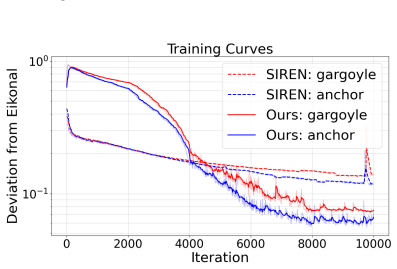
[Figure 5] Figure 5 lacks axis labels and a descriptive caption, making the reported 'Deviation from Eikonal' difficult to interpret.
[§A.4.2] The ablation text contains the typo '20/40/60/80%4 iterations'; it should read '80% iterations'.

Circularity Check

0 steps flagged · score 0.0 of 10

No circular steps found: ViscoReg is a self-contained regularizer, Theorem 1 is a genuine a priori bound in the minimized losses, and the viscosity theory used is external and classical.

full rationale

The derivation chain is self-contained. Theorem 1 bounds the infinity-norm error by the boundary and Eikonal training losses using external tools: the viscosity comparison principle (Lemma 1), a stability estimate (Lemma 2), and the Gagliardo-Nirenberg interpolation inequality. The residual functions f_{theta*} and g_{theta*} are defined from the trained network in Eq. 10, but this is a standard device for turning a PDE residual into a perturbed equation, and the theorem's conclusion is not identical to its input by construction. ViscoReg itself is a defined loss term, not a fitted parameter disguised as a prediction; the epsilon schedule is annealed and ablated rather than optimized against the reported test metrics. The only self-citation (Krishnan et al. 2025) appears in related work and is not load-bearing for any claim. Assumption 1 is explicitly stated as an assumption, and its failure mode is acknowledged, so it is a fragility rather than a circularity. The stability analysis in Sec. 4.2 (Eqs. 16-18) and the Lemma 2 proof in App. A.2.2 contain mathematical gaps, but these are correctness risks, not circular reductions: the paper does not define its conclusion in terms of its own fit or invoke an author-specific uniqueness theorem as the load-bearing step. Therefore no significant circularity is present.

Assumptions & free parameters 2 free parameters · 6 assumptions · 0 invented entities

The central claims rest on two domain assumptions (gradient bounded away from zero; quadrature accuracy), standard viscosity solution techniques, and one heuristic assumption in the linear stability analysis. No new entities are introduced.

free parameters (2)

viscosity coefficient epsilon = 0.5 to 0 (SRB, linear); 1.0 or 10.0 to 0 (ShapeNet, per category)
Annealed hyperparameter in the ViscoReg loss; schedule tuned per dataset and per shape category.
loss weights alpha_m, alpha_nm, alpha_e = [3000, 100, 50] (SRB, ShapeNet); [5000, 100, 50] (scene)
Hand-chosen weights for manifold, non-manifold, and Eikonal terms.

assumptions (6)

domain assumption Assumption 1: the network gradient is bounded away from zero: 0 < 1/C_theta* <= ||grad u_theta*|| <= C_theta*.
Invoked in Theorem 1 to apply Lemma 2; asserted to hold at a good local minimum but not proven. Section 3.3.
domain assumption Assumption 2: the sampled point cloud approximates continuous integrals with quadrature error O(N^-beta).
Used to replace L1 norms by discrete losses in Theorem 1. Section 3.3.
standard math Comparison principle and stability estimates for viscosity solutions of Hamilton-Jacobi equations.
Used in Lemmas 1 and 2. From Crandall and Lions 1983, Calder 2018.
standard math Gagliardo-Nirenberg interpolation inequality for bounded smooth domains.
Bridges L-infinity and L1 norms with W^(6,1) regularity in Theorem 1.
standard math The vanishing viscosity limit: solutions of ||grad u_epsilon||^2 = 1 + epsilon Delta u_epsilon converge uniformly to the viscosity solution of ||grad u||^2 = 1.
Motivates the ViscoReg loss; stated as Theorem 2 in appendix, cited to Crandall and Lions.
ad hoc to paper The sign of the residual, kappa_e = sign(1 + epsilon Delta u - ||grad u||^2), is treated as constant in the linearized Fourier analysis.
Heuristic assumption in the stability derivation (Eq. 17), not justified for the nonlinear PDE.

how reviews work

0 comments

Cite this review

Pith. "Pith review of ViscoReg: Neural Signed Distance Functions via Viscosity Solutions." pith.science (2026). https://pith.science/paper/ZKY4OIIF

@misc{pith2026250700412,
  author       = {Pith},
  title        = {Pith review of: ViscoReg: Neural Signed Distance Functions via Viscosity Solutions},
  year         = {2026},
  howpublished = {\url{https://pith.science/paper/ZKY4OIIF}},
  note         = {Machine review of arXiv:2507.00412}
}

read the original abstract

Implicit Neural Representations (INRs) that learn Signed Distance Functions (SDFs) from point cloud data represent the state-of-the-art for geometrically accurate 3D scene reconstruction. However, training these Neural SDFs often requires enforcing the Eikonal equation, an ill-posed equation that also leads to unstable gradient flows. Numerical Eikonal solvers have relied on viscosity approaches for regularization and stability. Motivated by this well-established theory, we introduce ViscoReg, a novel regularizer that provably stabilizes Neural SDF training. Empirically, ViscoReg outperforms state-of-the-art approaches such as SIREN, DiGS, and StEik on ShapeNet, the Surface Reconstruction Benchmark, and 3D scene reconstruction datasets. Additionally, we establish novel generalization error estimates for Neural SDFs in terms of the training error, using the theory of viscosity solutions.

Figures

Figures reproduced from arXiv: 2507.00412 by the authors.

**Figure 2.** Results from the scene reconstruction benchmark from Sitzmann et al. (2019b). The DiGS [PITH_FULL_IMAGE:figures/full_fig_p008_2.png] view at source ↗

**Figure 3.** Results from ShapeNet for examples drawn from the Chair (top left), Lamp (bottom right), [PITH_FULL_IMAGE:figures/full_fig_p009_3.png] view at source ↗

Figures from the paper (4 more)

**Figure 4.** Figure 4: Qualitative results from SRB [PITH_FULL_IMAGE:figures/full_fig_p019_4.png]

**Figure 5.** Figure 5: Deviation from Eikonal. 19 [PITH_FULL_IMAGE:figures/full_fig_p019_5.png]

**Figure 6.** Figure 6: Results from the scene reconstruction benchmark from Sitzmann et al. (2019b). The left [PITH_FULL_IMAGE:figures/full_fig_p020_6.png]

**Figure 7.** Figure 7: Quantitative results from the ShapeNet dataset from bench, cabinet, rifle and table cate [PITH_FULL_IMAGE:figures/full_fig_p022_7.png]

Discussion (0). Sign in to comment.

Reference graph

Works this paper leans on

18 extracted references · 9 canonical work pages

[2]

A.2 MATHEMATICALPROOFS Letu 1, u2 be viscosity solutions of∥∇u∥ 2 =f 1,∥∇u∥ 2 =f 2, respectively

Thenu ε →u uniformly, asε→0 +, whereεis the unique viscosity solution of (1). A.2 MATHEMATICALPROOFS Letu 1, u2 be viscosity solutions of∥∇u∥ 2 =f 1,∥∇u∥ 2 =f 2, respectively. The comparison principle states that iff 1 ≤f 2 in ¯Ω, andu 1|∂Ω ≤u 2|∂Ω thenu 1 ≤u 2 in ¯Ω. We prove Lemmas 1 and 2 using this theory (Calder, 2018). A.2.1 PROOF OFLEMMA1 LetC= max...

work page 2018
[7]

Chang et al

21 Under Review Figure 7: Quantitative results from the ShapeNet dataset from bench, cabinet, rifle and table cate- gories. Chang et al. (2015). 22

work page 2015
[9]

BL×x= baseline decay of 0.5/0.4/0.04/0.005/0 at 0/20/40/60/80%4iterations scaled byx

A.4.2 ABLATION For the ablation studies, the decay schedules are as follows. BL×x= baseline decay of 0.5/0.4/0.04/0.005/0 at 0/20/40/60/80%4iterations scaled byx. Fast decay corresponds to a quick decay to 0, of 0.5/0.0 at 0/20% iterations. Slow decay corresponds to extended decay at 90 percent of iterations with a schedule 0.5/0.4/0.04/0.005/0 at 0/20/40...

work page 2019
[10]

Define an auxillary function ˆuθ∗ ∈C( ¯Ω)such that it is the unique viscosity solution of the PDE: ∥∇ˆuθ∗ (x)∥2 = 1, x∈Ω,ˆu θ∗ (x) =g θ∗ (x), x∈∂Ω.(27) By the regularity of∂Ωandg θ∗ :∂Ω→R, we haveˆu θ∗ ∈C(Ω). Using the triangle inequality: ∥u−u θ∗ ∥∞ ≤ ∥u−ˆuθ∗ ∥∞ +∥ˆuθ∗ −u θ∗ ∥∞.(28) Using Lemma 1 and Lemma 2 to bound the first and second term, respective...

work page 1959
[11]

Neuralpde: Au- tomating physics-informed neural networks (pinns) with error approximations.arXiv preprint arXiv:2107.09443,

Kirill Zubov, Zoe McCarthy, Yingbo Ma, Francesco Calisto, Valerio Pagliarino, Simone Azeglio, Luca Bottero, Emmanuel Luj ´an, Valentin Sulzer, Ashutosh Bharambe, et al. Neuralpde: Au- tomating physics-informed neural networks (pinns) with error approximations.arXiv preprint arXiv:2107.09443,

arXiv
[12]

LetΩ⊆R n be an open, bounded domain and letu: Ω→Rbe a sufficiently regular function

A APPENDIX In this section, we provide supplementary details for our paper. LetΩ⊆R n be an open, bounded domain and letu: Ω→Rbe a sufficiently regular function. The following norms are defined (Evans, 2022). FUNCTIONSPACENORMS Lp NormFor1≤p <∞, theL p(Ω)norm is defined as: ∥u∥Lp(Ω) = Z Ω |u(x)|p dx 1/p Forp=∞, theL ∞(Ω)norm is defined by the essential sup...

work page 2022
[14]

Theorem 3LetΩ⊂R 3 be an open, smooth, bounded and connected domain

Consequently: ∥u1 −u 2∥L∞(Ω) ≤C ΩC −2 f ∥f1 −f 2∥∞ (25) 14 Under Review A.2.3 PROOF OFTHEOREM1 First, we state the following classical result that follows from the Gagliardo–Nirenberg interpolation inequality relating different function norms Nirenberg (1959). Theorem 3LetΩ⊂R 3 be an open, smooth, bounded and connected domain. Foru∈L 1(Ω)∩ W 6,1(Ω), we ha...

work page 1959
[16]

A.4 IMPLEMENTATIONDETAILS All the methods are evaluated on a single Nvidia RTX A6000 GPU

The gradient flow PDE ofL veik forp= 2takes the form: du dt =∇ ·((∥∇u∥2 −1) ∥∇u∥2 ∇u) +ε∆ ((∥∇u∥2 −1)∇u) +ε∇(∆u∇u)−ε 2∆(∆u)(34) Linearizing the PDE around the stationary linear solutionu=a·xgives the linear PDE: du dt =∂ 2 x1 u1 +ε∂ x1 (∆u)−ε 2∆(∆u) Taking the Fourier transform of this fourth order PDE: ˆu′(t) =−κ e|ω1|2 ˆu+iω3 1 ˆu−ε2|ω|4 ˆu=⇒ˆu(t) =e (−...

work page 1998

Show all 18 references

[1992]

Phase transitions, distance functions, and implicit neural representations.arXiv preprint arXiv:2106.07689,

Yaron Lipman. Phase transitions, distance functions, and implicit neural representations.arXiv preprint arXiv:2106.07689,

arXiv
[1998]

Neural-pull: Learning signed distance functions from point clouds by learning to pull space onto surfaces.arXiv preprint arXiv:2011.13495,

Baorui Ma, Zhizhong Han, Yu-Shen Liu, and Matthias Zwicker. Neural-pull: Learning signed distance functions from point clouds by learning to pull space onto surfaces.arXiv preprint arXiv:2011.13495,

2011 arXiv
[2006]

Shapenet: An information-rich 3d model repository.arXiv preprint arXiv:1512.03012,

Angel X Chang, Thomas Funkhouser, Leonidas Guibas, Pat Hanrahan, Qixing Huang, Zimo Li, Silvio Savarese, Manolis Savva, Shuran Song, Hao Su, et al. Shapenet: An information-rich 3d model repository.arXiv preprint arXiv:1512.03012,

arXiv
[2014]

SAL: Sign agnostic learning of shapes from raw data

Matan Atzmon and Yaron Lipman. SAL: Sign agnostic learning of shapes from raw data. In Proceedings of the IEEE/CVF conference on computer vision and pattern recognition, pp. 2565– 2574, 2020a. Matan Atzmon and Yaron Lipman. SALD: Sign agnostic learning with derivatives.arXiv p...

2006 arXiv
[2018]

When do ex- tended physics-informed neural networks (XPINNs) improve generalization?arXiv preprint arXiv:2109.09444,

Zheyuan Hu, Ameya D Jagtap, George Em Karniadakis, and Kenji Kawaguchi. When do ex- tended physics-informed neural networks (XPINNs) improve generalization?arXiv preprint arXiv:2109.09444,

arXiv
[2020]

A survey and benchmark of automatic surface reconstruction from point clouds.IEEE Trans

Raphael Sulzer, Renaud Marlet, Bruno Vallet, and Loic Landrieu. A survey and benchmark of automatic surface reconstruction from point clouds.IEEE Trans. Pattern Anal. Mach. Intell., PP(3):2000–2019, December

2000
[2021]

Neural volumes: Learning dynamic renderable volumes from images.arXiv preprint arXiv:1906.07751,

Stephen Lombardi, Tomas Simon, Jason Saragih, Gabriel Schwartz, Andreas Lehrmann, and Yaser Sheikh. Neural volumes: Learning dynamic renderable volumes from images.arXiv preprint arXiv:1906.07751,

1906 arXiv
[2022]

Implicit geometric regu- larization for learning shapes.arXiv preprint arXiv:2002.10099,

Amos Gropp, Lior Yariv, Niv Haim, Matan Atzmon, and Yaron Lipman. Implicit geometric regu- larization for learning shapes.arXiv preprint arXiv:2002.10099,

2002 arXiv
[2023]

3d gaussian splatting with normal information for mesh extraction and improved rendering.arXiv preprint arXiv:2501.08370,

Meenakshi Krishnan, Liam Fowl, and Ramani Duraiswami. 3d gaussian splatting with normal information for mesh extraction and improved rendering.arXiv preprint arXiv:2501.08370,

arXiv
[2024]

doi: 10.1109/TPAMI.2024

ISSN 0162-8828,1939-3539. doi: 10.1109/TPAMI.2024. 3510932. URLhttp://dx.doi.org/10.1109/TPAMI.2024.3510932. Joanna Waczy´nska, Piotr Borycki, Sławomir Tadeja, Jacek Tabor, and Przemysław Spurek. Games: Mesh-based adapting and modification of gaussian splatting.arXiv preprint ...

1939

Pith tools

Reviewed August 6, 2026 · model on record in the stance chip above.

[1] [2]

A.2 MATHEMATICALPROOFS Letu 1, u2 be viscosity solutions of∥∇u∥ 2 =f 1,∥∇u∥ 2 =f 2, respectively

Thenu ε →u uniformly, asε→0 +, whereεis the unique viscosity solution of (1). A.2 MATHEMATICALPROOFS Letu 1, u2 be viscosity solutions of∥∇u∥ 2 =f 1,∥∇u∥ 2 =f 2, respectively. The comparison principle states that iff 1 ≤f 2 in ¯Ω, andu 1|∂Ω ≤u 2|∂Ω thenu 1 ≤u 2 in ¯Ω. We prove Lemmas 1 and 2 using this theory (Calder, 2018). A.2.1 PROOF OFLEMMA1 LetC= max...

work page 2018

[2] [7]

Chang et al

21 Under Review Figure 7: Quantitative results from the ShapeNet dataset from bench, cabinet, rifle and table cate- gories. Chang et al. (2015). 22

work page 2015

[3] [9]

BL×x= baseline decay of 0.5/0.4/0.04/0.005/0 at 0/20/40/60/80%4iterations scaled byx

A.4.2 ABLATION For the ablation studies, the decay schedules are as follows. BL×x= baseline decay of 0.5/0.4/0.04/0.005/0 at 0/20/40/60/80%4iterations scaled byx. Fast decay corresponds to a quick decay to 0, of 0.5/0.0 at 0/20% iterations. Slow decay corresponds to extended decay at 90 percent of iterations with a schedule 0.5/0.4/0.04/0.005/0 at 0/20/40...

work page 2019

[4] [10]

Define an auxillary function ˆuθ∗ ∈C( ¯Ω)such that it is the unique viscosity solution of the PDE: ∥∇ˆuθ∗ (x)∥2 = 1, x∈Ω,ˆu θ∗ (x) =g θ∗ (x), x∈∂Ω.(27) By the regularity of∂Ωandg θ∗ :∂Ω→R, we haveˆu θ∗ ∈C(Ω). Using the triangle inequality: ∥u−u θ∗ ∥∞ ≤ ∥u−ˆuθ∗ ∥∞ +∥ˆuθ∗ −u θ∗ ∥∞.(28) Using Lemma 1 and Lemma 2 to bound the first and second term, respective...

work page 1959

[5] [11]

Neuralpde: Au- tomating physics-informed neural networks (pinns) with error approximations.arXiv preprint arXiv:2107.09443,

Kirill Zubov, Zoe McCarthy, Yingbo Ma, Francesco Calisto, Valerio Pagliarino, Simone Azeglio, Luca Bottero, Emmanuel Luj ´an, Valentin Sulzer, Ashutosh Bharambe, et al. Neuralpde: Au- tomating physics-informed neural networks (pinns) with error approximations.arXiv preprint arXiv:2107.09443,

arXiv

[6] [12]

LetΩ⊆R n be an open, bounded domain and letu: Ω→Rbe a sufficiently regular function

A APPENDIX In this section, we provide supplementary details for our paper. LetΩ⊆R n be an open, bounded domain and letu: Ω→Rbe a sufficiently regular function. The following norms are defined (Evans, 2022). FUNCTIONSPACENORMS Lp NormFor1≤p <∞, theL p(Ω)norm is defined as: ∥u∥Lp(Ω) = Z Ω |u(x)|p dx 1/p Forp=∞, theL ∞(Ω)norm is defined by the essential sup...

work page 2022

[7] [14]

Theorem 3LetΩ⊂R 3 be an open, smooth, bounded and connected domain

Consequently: ∥u1 −u 2∥L∞(Ω) ≤C ΩC −2 f ∥f1 −f 2∥∞ (25) 14 Under Review A.2.3 PROOF OFTHEOREM1 First, we state the following classical result that follows from the Gagliardo–Nirenberg interpolation inequality relating different function norms Nirenberg (1959). Theorem 3LetΩ⊂R 3 be an open, smooth, bounded and connected domain. Foru∈L 1(Ω)∩ W 6,1(Ω), we ha...

work page 1959

[8] [16]

A.4 IMPLEMENTATIONDETAILS All the methods are evaluated on a single Nvidia RTX A6000 GPU

The gradient flow PDE ofL veik forp= 2takes the form: du dt =∇ ·((∥∇u∥2 −1) ∥∇u∥2 ∇u) +ε∆ ((∥∇u∥2 −1)∇u) +ε∇(∆u∇u)−ε 2∆(∆u)(34) Linearizing the PDE around the stationary linear solutionu=a·xgives the linear PDE: du dt =∂ 2 x1 u1 +ε∂ x1 (∆u)−ε 2∆(∆u) Taking the Fourier transform of this fourth order PDE: ˆu′(t) =−κ e|ω1|2 ˆu+iω3 1 ˆu−ε2|ω|4 ˆu=⇒ˆu(t) =e (−...

work page 1998