REVIEW 2 major objections 5 minor 57 references
Bounce-Averaged Theory In Arbitrary Multi-Well Plasmas: Solution Domains and the Graph Structure of their Connections
T0 review · 2 major / 5 minor · reviewed 2026-08-06 · deepseek-v4-flash
Pith's one-line read A set of compatibility rules determines all solution domains and boundary connections needed to run bounce-averaged Fokker-Planck simulations in arbitrarily complicated multi-well plasma geometries.
desk verdict A genuinely useful algorithmic framework for multi-well bounce-averaged domains, but the boundary conditions as written miss the √g_Z factor and the domain-summary claim overreaches. read the letter →
The pith
A machine-rendered reading of the paper's core claim, the machinery that carries it, and where it could break.
The reading
What carries the argument
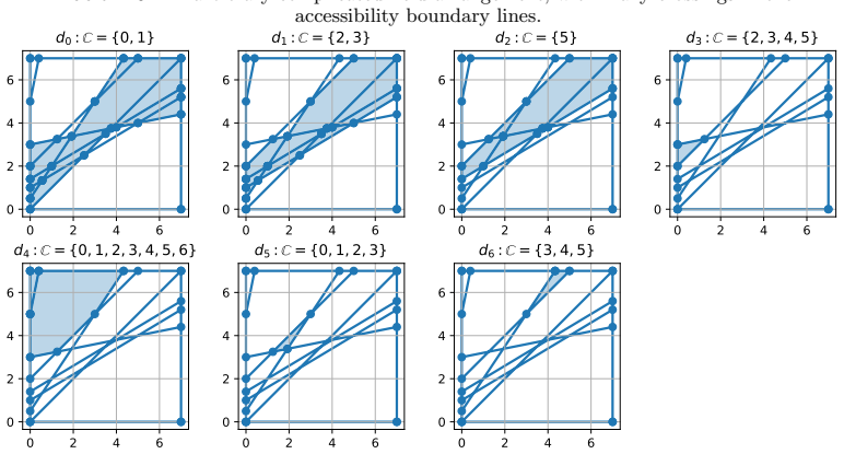
The central object is the population: a region $r_i$ of $(\epsilon,\mu)$ COM space paired with a maximal continuous subsequence $C^m_i$ of allowed axial segments. The argument reduces trajectory identity to which contiguous block of axial segments a particle can reach, and the load-bearing conditions are connectedness (4.2) and reciprocal uniqueness (4.3)-(4.4), which together ensure that moving across a region boundary does not silently merge or split trajectories in a way that would make the distribution multivalued. The directed graph built from these connections, with edges running from the region whose allowed segment set is a strict superset (higher access) to the lower-access region, is the concise visual encoding of the trajectory bifurcation structure.
What would settle it
Run full-orbit simulations for the Appendix A field configuration with $a_B>a_\psi$ and check whether every trajectory with $(\epsilon,\mu)$ in the bifurcated region stays forever inside exactly one maximal contiguous segment block. Any orbit that switches blocks without crossing the predicted domain boundary in COM space, or any pair of distinct trajectories with identical $(\epsilon,\mu)$ and the same segment block, would falsify the one-to-one mapping that the domain construction relies on.
Extended reading notes
Core claim
The paper's central claim is that for any set of axial segments with accessibility condition $\epsilon \geq \mu B(n)+\psi(n)$, the compatibility conditions (4.2)-(4.4) together with the boundary rules (5.2)-(5.5) are sufficient to partition COM space into consistent domains, so that within each domain a point $Z=(\epsilon,\mu)$ corresponds to exactly one trajectory and particle conservation holds across every internal boundary. The construction first splits $(\epsilon,\mu)$ space into regions bounded by the curves $\epsilon=\mu B(n)+\psi(n)$, then defines a population as a region paired with one maximal continuous subsequence of allowed axial segments, and groups populations into domains by requiring pairwise compatibility and connectedness. The paper shows that the compatibility relation is not transitive and that the decomposition is not unique, and it supplies an explicit algorithm (Appendix C) for producing a valid decomposition. If correct, this makes bounce-averaged simulations feasible for arbitrarily complicated, dynamically evolving electromagnetic geometries.
Load-bearing premise
The method rests on assuming that a particle's trajectory is fully determined by which maximal contiguous block of axial segments it can reach at a given $(\epsilon,\mu)$, which requires the fast gyro-bounce motion to be exactly adiabatic and one-dimensional along the field line, with no additional invariants or chaotic behavior.
Editorial extensions
If this is right
- Bounce-averaged Fokker-Planck codes can be set up automatically, without hand-identifying wells, even when the fields and their potential maxima change during the simulation.
- The same compatibility conditions apply in three-dimensional COM space $(\epsilon,\mu,\Phi)$, where region boundaries become two-dimensional surfaces rather than curves.
- The directed graph of domain connections tells the solver exactly which boundary conditions to apply at each shared surface, and reduces to reflecting conditions where no connected population exists.
- The framework applies beyond mirrors to any plasma with well-defined constants of motion, including tokamaks and quasisymmetric stellarators.
- Because the domain decomposition is not unique, a code can choose among equally valid partitions, leaving room to optimize for numerical efficiency or smoothness.
Reading between the lines
- Editorial: the same population-and-domain decomposition could be used to bounce-average any orbit-integrated operator, not only Fokker-Planck fluxes, such as synchrotron emission, radiation absorption, or quasilinear diffusion coefficients, because the averaging step is identical.
- Editorial: the non-uniqueness of the decomposition suggests a design problem the paper does not solve: choose the valid partition that minimizes interface count or numerical diffusion for a given grid.
- Editorial: the adiabatic one-dimensional assumption could be stress-tested by comparing the graph's predicted connectivity against full-orbit integrations in a 3D field with magnetic shear or mirror asymmetries; trajectories that change segment block without crossing a domain boundary would invalidate the mapping.
Editorial analysis
A structured set of objections, weighed in public.
Referee Report
Summary. This paper addresses the problem of defining solution domains for bounce-averaged Fokker-Planck (BAFP) calculations when the constants of motion do not uniquely specify a particle trajectory because of multiple wells in the magnetic or electric potential. The author introduces a combinatorial construction on a discretized field line: for each region of COM space, compute the set of axial segments accessible to a particle, split this set into maximal continuous subsequences (populations), group populations into domains using connectedness and pairwise compatibility conditions (4.2)-(4.4), and stitch domains together with continuity and flux-matching boundary conditions (5.2)-(5.5). The domain-connection structure is represented as a directed graph. Worked examples include a double well, a Yushmanov-trapped case, a tiered well, and an arbitrary field arrangement, together with a proposed algorithm for automated decomposition (Appendix C).
Significance. If correct, the paper would fill a practical gap: current BAFP codes impose multi-well domain structures by hand, and modern mirror designs with self-consistent kinetic potentials need automatic detection. The main contribution is the formalization of populations and domains, the explicit boundary-matching rules, and the graph encoding of trajectory bifurcations. The paper also gives a neat differential criterion for Yushmanov trajectory bifurcation (Appendix A). Strengths include the explicit, parameter-free construction, the detailed worked examples, and the algorithmic procedure in Appendix C, which should be directly useful for code development. However, the boundary-condition formulation has a load-bearing gap concerning the bounce-averaged volume element in the flux matching, and the paper would benefit from a numerical flux-balance test on one example. The 3D generalization is asserted rather than demonstrated, a limitation that should be stated clearly.
major comments (2)
- [Sec. 5, Eqs. (5.3) and (5.5); Sec. 3, Eq. (3.2)] The flux-matching conditions equate n_i Gamma^i_Z across a boundary, but the conservative flux in the bounce-averaged equation (2.11) is sqrt(g_Z) Gamma^i_Z, not Gamma^i_Z. Equation (2.13) defines Gamma^i_Z with an explicit factor 1/sqrt(g_Z), so Gamma^i_Z is the orbit-averaged flux operator, not the conservative flux. At a boundary between a higher-access domain and a lower-access domain, the bounce-averaged volume element sqrt(g_Z) is computed over different axial segment sets and is generally different; at a separatrix it can diverge, with different finite parts on the two sides. Equating only n_i Gamma^i_Z therefore does not enforce conservation of the physical flux sqrt(g_Z) Gamma^i_Z. The matching condition should read n_i (sqrt(g_Z) Gamma^i_Z)|_{d_a} = sum_{d_b} n_i (sqrt(g_Z) Gamma^i_Z)|_{d_b}, with each term evaluated in the appropriate domain. Because particle conservation across domain boundaries is one of the central claims of the paper, this is a substantive issue rather than a typographical one. I recommend adding a small numerical flux-balance check to one of the examples to confirm the corrected condition.
- [Sec. 4 and Appendix C] The paper claims that the conditions (4.2)-(4.4) are sufficient to set up a well-posed BAFP problem, but it does not prove that every maximal domain produced by the algorithm has the property that f is single-valued on it, in particular that a domain cannot contain two populations in the same region with different C_m^i. The algorithm in Appendix C step (vii) explicitly avoids adding a second population from a region already in the domain, so the constructive procedure is safe; however, the broader sufficiency statement in Sec. 6 goes beyond the algorithm. Either prove that pairwise compatibility rules out duplicate-region populations in any connected domain, or restrict the sufficiency claim to the output of the constructive algorithm.
minor comments (5)
- [Eq. (5.5)] The right-hand side of Eq. (5.5) repeats the left-hand side's boundary and domain labels; it should sum over d_c in D^b_ji with the corresponding boundary labels (e.g., b^c_ij,d_c), otherwise the equation is not the intended matching condition.
- [Appendix B] The population p0_3 is listed as being in region r2, but the surrounding text refers to it as in region r3; the figure suggests r3, so one of these is a typo.
- [Throughout] There are several typographical errors, including 'cosistent' in the Sec. 4 heading, 'attempted' in Sec. 3.1, 'distrbutions' in Sec. 7, 'acessibility' in figure captions, and 'arbitary' in Secs. 1 and 7.
- [Sec. 4, first paragraph] The statement that the generalization to 3D COM space is 'straightforward' is an assertion; the paper does not address 3D-specific issues such as the dependence of B and psi on the flux coordinate, possible tangencies of the boundary surfaces, or the role of non-axisymmetric geometries. State the assumptions (axisymmetry, adiabaticity, no additional invariants) more prominently.
- [Appendix B] The non-uniqueness example is valid, but I checked that it does not contradict the Sec. 4 claim that each domain has a single continuous set of axial segments C_a: in the two decompositions shown, the unions of the C sets are {0,1,2} and {0,1}, both of which are contiguous.
Circularity Check
No significant circularity: the domain-construction rules are explicitly presented as a formalization/definitional framework, not fitted predictions, and no load-bearing self-citation forces the conclusion.
full rationale
The paper's central contribution is a formalization: populations are defined as (region, maximal continuous axial-subsequence) pairs, and domains are defined as connected, pairwise-compatible collections of populations (Sec. 4). The conditions (4.2)-(4.4) are operative definitions of connectedness and compatibility, and the boundary conditions (5.2)-(5.5) are direct statements of continuity and flux matching in the bounce-averaged equation. There is no fitted parameter that is later renamed a prediction, and no empirical quantity is being recovered from an input. The Yushmanov-trajectory bifurcation condition (3.4)/(A 7)/(A 8) is derived from the accessibility inequalities by a Taylor expansion, not imported from a prior result. The cited prior work by the author (e.g., Kolmes et al. 2024 for the rotating-frame potential, Ochs et al. 2023 for ambipolar potentials, Ochs et al. 2024/2025 for radiation and ash effects) is contextual and not load-bearing for the domain-construction theorem. The paper also explicitly acknowledges non-uniqueness of the domain decomposition (Appendix B), which would be odd for a claim that the answer is forced by a self-citation chain. The main physical assumption—that each trajectory is identified by its set of accessible axial segments—is stated as a starting point rather than derived, which is an assumption and a possible correctness limitation, but not circularity. The reviewer-identified omission of sqrt(g_Z) factors in the flux-matching conditions (3.2)/(5.3)/(5.5) is a potential internal inconsistency or correctness issue in the boundary conditions, but it is not a circular reduction of a prediction to an input. Overall, the derivation chain is self-contained against the paper's stated definitions and assumptions.
Assumptions & free parameters
assumptions (5)
- domain assumption The fast particle motion is exactly periodic with conserved constants of motion (epsilon, mu, Phi), and f is independent of gyro angle, azimuthal angle, and field-line coordinate after averaging.
- domain assumption A particle can access axial segment n iff epsilon >= mu B(n)+psi(n), and its trajectory visits exactly one maximal continuous subsequence of the accessible segments.
- domain assumption Fields are piecewise constant along the field line; the continuum limit Delta s to 0 is assumed to recover the continuous theory.
- ad hoc to paper The generalization from 2D (epsilon, mu) to 3D (epsilon, mu, Phi) COM space is straightforward and needs no separate proof.
- domain assumption At internal boundaries, continuity of f and flux conservation are the correct matching conditions; external loss-cone boundaries are absorbing and kinetic-energy boundaries are reflecting.
Cite this review
Pith. "Pith review of Bounce-Averaged Theory In Arbitrary Multi-Well Plasmas: Solution Domains and the Graph Structure of their Connections." pith.science (2026). https://pith.science/paper/I6O62XSA
@misc{pith2026250700778,
  author       = {Pith},
  title        = {Pith review of: Bounce-Averaged Theory In Arbitrary Multi-Well Plasmas: Solution Domains and the Graph Structure of their Connections},
  year         = {2026},
  howpublished = {\url{https://pith.science/paper/I6O62XSA}},
  note         = {Machine review of arXiv:2507.00778}
}
read the original abstract
Bounce-averaged theories provide a framework for simulating relatively slow processes, such as collisional transport and quasilinear diffusion, by averaging these processes over the fast periodic motions of a particle on a closed orbit. This procedure dramatically increases the characteristic timescale and reduces the dimensionality of the modeled system. The natural coordinates for such calculations are the constants of motion (COM) of the fast particle motion, which by definition do not change during an orbit. However, for sufficiently complicated fields -- particularly in the presence of local maxima of the electric potential and magnetic field -- the COM are not sufficient to specify the particle trajectory. In such cases, multiple domains in COM space must be used to solve the problem, with boundary conditions enforced between the domains to ensure continuity and particle conservation. Previously, these domains have been imposed by hand, or by recognizing local maxima in the fields, limiting the flexibility of bounce-averaged simulations. Here, we present a general set of conditions for identifying consistent domains and the boundary condition connections between the domains, allowing the application of bounce-averaged theories in arbitrarily complicated and dynamically-evolving electromagnetic field geometries. We also show how the connections between the domains can be represented by a directed graph, which can help to succinctly represent the trajectory bifurcation structure.
Figures


Figures from the paper (11 more)




Reference graph
Works this paper leans on
-
[1]
Be'ery, I. , Gertsman, A. & Seeman, O. 2018 Plasma confinement by moving multiple mirrors . Plasma Physics and Controlled Fusion 60 (11), 115004
work page 2018
-
[2]
Bekhtenev, A. , Volosov, V. , Pal'chikov, V. , Pekker, M. & Yudin, Yu.N . 1980 Problems of a thermonuclear reactor with a rotating plasma . Nuclear Fusion 20 (5), 579--598
work page 1980
-
[3]
BenDaniel, D. J. & Allis, W. P. 1962 Scattering loss from magnetic mirror systems - II . Journal of Nuclear Energy. Part C, Plasma Physics, Accelerators, Thermonuclear Research 4 (2), 79--88
work page 1962
-
[4]
Bernstein, I. B. & Baxter, D. C. 1981 Relativistic theory of electron cyclotron resonance heating . The Physics of Fluids 24 (1), 108--126
work page 1981
-
[5]
Bilbao, P. J. & Silva, L. O. 2023 Radiation Reaction Cooling as a Source of Anisotropic Momentum Distributions with Inverted Populations . Physical Review Letters 130 (16), 165101
work page 2023
-
[6]
Cho, T. , Yoshida, M. , Kohagura, J. , Hirata, M. , Numakura, T. , Higaki, H. , Hojo, H. , Ichimura, M. , Ishii, K. , Islam, K. Md . , Itakura, A. , Katanuma, I. , Nakashima, Y. , Saito, T. , Tatematsu, Y. , Yoshikawa, M. , Kojima, Y. , Tokioka, S. , Yokoyama, N. , Tomii, Y. , Imai, T. , Pastukhov, V. P. & Miyoshi, S. 2005 Observation of the Effects of Ra...
work page 2005
-
[7]
Cohen, R. H. , Bernstein, I. B. , Dorning, J. J. & Rowlands, G. 1980 Particle and energy exchange between untrapped and electrostatically confined populations in magnetic mirrors . Nuclear Fusion 20 (11), 1421--1437
work page 1980
-
[8]
d'Herbemont , V. , Parra, F. I. , Calvo, I. & Velasco, J. L. 2022 Finite orbit width effects in large aspect ratio stellarators . Journal of Plasma Physics 88 (5), 905880507
work page 2022
Show all 57 references
-
[9]
, Endrizzi, D
Egedal, J. , Endrizzi, D. , Forest, C. & Fowler, T. 2022 Fusion by beam ions in a low collisionality, high mirror ratio magnetic mirror . Nuclear Fusion 62 (12), 126053
2022
-
[10]
, Anderson, J
Endrizzi, D. , Anderson, J. K. , Brown, M. , Egedal, J. , Geiger, B. , Harvey, R. W. , Ialovega, M. , Kirch, J. , Peterson, E. , Petrov, Y. V. , Pizzo, J. , Qian, T. , Sanwalka, K. , Schmitz, O. , Wallace, J. , Yu, M. & Forest, C. B. 2023 Physics basis for the Wisconsin HTS Ax...
2023
-
[11]
& Helander, P
Eriksson, L.-G. & Helander, P. 1994 Monte Carlo operators for orbit-averaged Fokker -- Planck equations . Physics of Plasmas 1 (2), 308--314
1994
-
[12]
Fisch, N. J. 1987 Theory of current drive in plasmas . Reviews of Modern Physics 59 (1), 175--234
1987
-
[13]
Fisch, N. J. & Rax, J.-M. 1992 Interaction of energetic alpha particles with intense lower hybrid waves . Physical Review Letters 69 (4), 612--615
1992
-
[14]
, Moir, R
Fowler, T. , Moir, R. & Simonen, T. 2017 A new simpler way to obtain high fusion power gain in tandem mirrors . Nuclear Fusion 57 (5), 056014
2017
-
[15]
Frank, S. J. , Viola, J. , Petrov, Y. V. , Anderson, J. K. , Bindl, D. , Biswas, B. , Caneses, J. , Endrizzi, D. , Furlong, K. , Harvey, R. W. , Jacobson, C. M. , Lindley, B. , Marriott, E. , Schmitz, O. , Shih, K. & Forest, C. B. 2024 Integrated modelling of equilibrium and t...
2024
-
[16]
, Yoon, E
Hager, R. , Yoon, E. , Ku, S. , D'Azevedo, E. , Worley, P. & Chang, C. 2016 A fully non-linear multi-species Fokker -- Planck -- Landau collision operator for simulation of fusion plasma . Journal of Computational Physics 315 , 644--660
2016
-
[17]
& McCoy, MG
Harvey, RW . & McCoy, MG . 1992 The CQL3D fokker-planck code. In Proceedings of the IAEA Technical Committee Meeting on Simulation and Modeling of Thermonuclear Plasmas\/ , pp. 489--526
1992
-
[18]
Herrmann, M. C. 1998 Cooling Alpha Particles With Waves . PhD thesis, Princeton
1998
-
[19]
Herrmann, M. C. & Fisch, N. J. 1997 Cooling Energetic Alpha Particles in a Tokamak with Waves . Physical Review Letters 79 (8), 1495--1498
1997
-
[20]
, Kiwamoto, Y
Katanuma, I. , Kiwamoto, Y. , Ishii, K. & Miyoshi, S. 1986 Thermal barrier potential of a tandem mirror . Physics of Fluids 29 (12), 4138
1986
-
[21]
, Kiwamoto, Y
Katanuma, I. , Kiwamoto, Y. , Sawada, K. & Miyoshi, S. 1987 Fokker-- Planck calculation of hot electron buildup in the thermal barrier region of a tandem mirror . Physics of Fluids 30 (4), 1142
1987
-
[22]
Kolmes, E. J. & Fisch, N. J. 2024 Coriolis forces modify magnetostatic ponderomotive potentials . Physics of Plasmas 31 (11), 112107
2024
-
[23]
Kolmes, E. J. , Ochs, I. E. & Fisch, N. J. 2025 Ion Mix Can Invert Centrifugal Traps , arXiv:arXiv: 2504.18634
2025
-
[24]
Kolmes, E. J. , Ochs, I. E. , Rax, J.-M. & Fisch, N. J. 2024 Massive, long-lived electrostatic potentials in a rotating mirror plasma . Nature Communications 15 (1), 4302
2024
-
[25]
, Landman, IS
Konkashbaev, IK . , Landman, IS . & Ulinich, FR . 1978 Possibility of decreasing the electron heat flux from open traps . Soviet Physics JETP 47 , 501
1978
-
[26]
Marx, K. D. 1970 Effects of Spatial Variations on Collisional Losses in a Mirror-Confined Plasma . The Physics of Fluids 13 (5), 1355--1371
1970
-
[27]
& Stewart, J
Matsuda, Y. & Stewart, J. 1986 A relativistic multiregion bounce-averaged Fokker-Planck code for mirror plasmas . Journal of Computational Physics 66 (1), 197--217
1986
-
[28]
, Be'ery, I
Miller, T. , Be'ery, I. & Barth, I. 2021 Rate equations model for multiple magnetic mirrors in various thermodynamic scenarios . Physics of Plasmas 28 (11), 112506
2021
-
[29]
, Be'ery, I
Miller, T. , Be'ery, I. , Gudinetsky, E. & Barth, I. 2023 RF plugging of multi-mirror machines . Physics of Plasmas 30 (7), 072510
2023
-
[30]
Mirnov, V. V. & Riutov, D. D. 1979 Linear gasdynamic system for plasma confinement . Technical Physics Letters 5 , 279
1979
-
[31]
& Hitchon, W
Mynick, H. & Hitchon, W. 1986 A bounce-averaged Fokker-Planck code for stellarator transport . Nuclear Fusion 26 (4), 425--438
1986
-
[32]
, Conn, R
Najmabadi, F. , Conn, R. & Cohen, R. 1984 Collisional end loss of electrostatically confined particles in a magnetic mirror field . Nuclear Fusion 24 (1), 75--84
1984
-
[33]
Nemov, V. V. , Kasilov, S. V. , Kernbichler, W. & Heyn, M. F. 1999 Evaluation of 1/ neoclassical transport in stellarators . Physics of Plasmas 6 (12), 4622--4632
1999
-
[34]
Ochs, I. E. 2024 Synchrotron-driven Instabilities in Relativistic Plasmas of Arbitrary Opacity . The Astrophysical Journal 975 (1), 30
2024
-
[35]
Ochs, I. E. & Fisch, N. J. 2023 Critical role of isopotential surfaces for magnetostatic ponderomotive forces . Physical Review E 108 (6), 065210
2023
-
[36]
Ochs, I. E. , Kolmes, E. J. & Fisch, N. J. 2025 Preventing ash from poisoning proton-boron 11 fusion plasmas
2025
-
[37]
Ochs, I. E. , Mlodik, M. E. & Fisch, N. J. 2024 Electron tail suppression and effective collisionality due to synchrotron emission and absorption in mildly relativistic plasmas . Physics of Plasmas 31 (8), 083303
2024
-
[38]
Ochs, I. E. , Munirov, V. R. & Fisch, N. J. 2023 Confinement time and ambipolar potential in a relativistic mirror-confined plasma . Physics of Plasmas 30 (5), 052508
2023
-
[39]
1974 Collisional losses of electrons from an adiabatic trap in a plasma with a positive potential
Pastukhov, V. 1974 Collisional losses of electrons from an adiabatic trap in a plasma with a positive potential . Nuclear Fusion 14 (1), 3--6
1974
-
[40]
1987 The magnetic mirror approach to fusion
Post, R. 1987 The magnetic mirror approach to fusion . Nuclear Fusion 27 (10), 1579--1739
1987
-
[41]
Rax, J. M. , Fruchtman, A. , Gueroult, R. & Fisch, N. J. 2015 Breakdown of the Brillouin limit and classical fluxes in rotating collisional plasmas . Physics of Plasmas 22 (9), 092101
2015
-
[42]
& Cutler, T
Rognlien, T. & Cutler, T. 1980 Transition from Pastukhov to collisional confinement in a magnetic and electrostatic well . Nuclear Fusion 20 (8), 1003--1011
1980
-
[43]
Rosenbluth, M. N. , MacDonald, W. M. & Judd, D. L. 1957 Fokker- Planck Equation for an Inverse-Square Force . Physical Review 107 (1), 1--6
1957
-
[44]
& Fisch, N
Rubin, T. & Fisch, N. J. 2025 Ponderomotive barriers in rotating mirror devices using static fields, arXiv:arXiv: 2502.02008
2025 arXiv
-
[45]
, Ochs, I
Rubin, T. , Ochs, I. E. & Fisch, N. J. 2024 Flowing plasma rearrangement in the presence of static perturbing fields . Physics of Plasmas 31 (8), 082109
2024
-
[46]
, Rax, J
Rubin, T. , Rax, J. M. & Fisch, N. J. 2023 Magnetostatic ponderomotive potential in rotating plasma . Physics of Plasmas 30 (5), 052501
2023
-
[47]
Schwartz, N. R. , Abel, I. G. , Hassam, A. B. , Kelly, M. & Romero-Talam \'a s , C. A. 2024 MCTrans ++: A 0- D model for centrifugal mirrors . Journal of Plasma Physics 90 (2), 905900217
2024
-
[48]
Skovorodin, D. I. 2019 Suppression of secondary emission of electrons from end plate in expander of open trap . Physics of Plasmas 26 (1), 012503
2019
-
[49]
1975 Fast-wave heating of a two-component plasma
Stix, T. 1975 Fast-wave heating of a two-component plasma . Nuclear Fusion 15 (5), 737--754
1975
-
[50]
, Calvo, I
Velasco, J. , Calvo, I. , Parra, F. & Garc \'i a-Rega \ n a , J. 2020 KNOSOS : A fast orbit-averaging neoclassical code for stellarator geometry . Journal of Computational Physics 418 , 109512
2020
-
[51]
Yushmanov, E. E. 1966 Confinement of Slow Ions of a Plasma with Positive Potential in a Mirror Trap . Soviet Physics JETP 22 , 409
1966
-
[52]
, Kunz, M
Zhdankin, V. , Kunz, M. W. & Uzdensky, D. A. 2023 Synchrotron Firehose Instability . The Astrophysical Journal 944 (1), 24
2023
-
[53]
, " * write output.state after.block = add.period write newline
ENTRY address author booktitle chapter edition editor howpublished institution journal key month note number organization pages publisher school series title type volume year eprint label extra.label sort.label short.list INTEGERS output.state before.all mid.sentence after.sen...
-
[54]
write newline
" write newline "" before.all 'output.state := FUNCTION n.dashify 't := "" t empty not t #1 #1 substring "-" = t #1 #2 substring "--" = not "--" * t #2 global.max substring 't := t #1 #1 substring "-" = "-" * t #2 global.max substring 't := while if t #1 #1 substring * t #2 gl...
-
[55]
@esa (Ref
\@ifclassloaded aguplus natbib The aguplus class already includes natbib coding, so you should not add it explicitly Type <Return> for now, but then later remove the command natbib from the document \@ifclassloaded nlinproc natbib The nlinproc class already includes natbib cod...
-
[56]
@stdbsttrue NAT@ctr \@lbibitem[ NAT@ctr ] \@lbibitem[#1]#2 \@extra@b@citeb \@ifundefined br@#2\@extra@b@citeb \@namedef br@#2 \@nameuse br@#2\@extra@b@citeb \@ifundefined b@#2\@extra@b@citeb @num @parse #2 [ @natanchorstart #2\@extra@b@citeb \@biblabel @num @natanchorend] @ifc...
-
[57]
@open @close @open @close and [1] URL: #1 \@ifundefined chapter * \@mkboth \@ifundefined NAT@sectionbib * \@mkboth * \@mkboth\@gobbletwo \@ifclassloaded amsart * \@ifclassloaded amsbook * \@ifundefined bib@heading @heading NAT@ctr thebibliography [1] @ \@biblabel NAT@ctr \@bib...
1996
Reviewed August 6, 2026 · model on record in the stance chip above.
Discussion (0). Continue with ORCID to comment.