REVIEW 4 major objections 4 minor 52 references
A Stable and Theoretically Grounded Gromov-Wasserstein Distance for Reeb Graph Comparison using Persistence Images
T0 review · 4 major / 4 minor · reviewed 2026-08-06 · deepseek-v4-flash
Pith's one-line read A new Reeb graph distance provably tracks scalar-field perturbations.
desk verdict The RGWp framework is a sensible, well-tested combination of existing ideas, but the advertised stability theorem rests on an unproved node-bijection assumption that is itself a stability claim; the paper deserves a serious referee but not acceptance as-is. read the letter →
The pith
A machine-rendered reading of the paper's core claim, the machinery that carries it, and where it could break.
The reading
What carries the argument
The load-bearing construction is the decorated Reeb graph $R^*_f=(R_f,d_{R_f},\nu_{R_f})$. The metric $d_{R_f}(v,u)=\tfrac12(\rho_f(v,u)+\rho_f(u,v))$ symmetrizes the Reeb radius, giving a genuine metric that tracks functional variation along graph paths without the asymmetry of the raw Reeb radius or the noise sensitivity of shortest-path distances. The measure $\nu_{R_f}$ is obtained by converting the extended persistence diagram into a persistence image, reading off each node's contribution as a Gaussian evaluation of that image at the node's birth-persistence point, and normalizing; this encodes how central each node is to the field's persistent features. The stability proof chains four estimates: bottleneck stability of extended persistence diagrams, $L^1$ stability of persistence images, total-variation stability of the normalized node measures, and Mémoli's inequality relating $\mathrm{RGW}_p$ to the Gromov-Prokhorov distance.
What would settle it
Take two scalar fields with arbitrarily small sup-norm difference whose Reeb graphs have different numbers of significant vertices (for instance, a persistence pair whose birth and death values cross under the perturbation), then compute the total-variation distance between their persistence-image node measures; if this distance does not go to zero as $\|f-g\|_\infty$ goes to zero, the measure-stability step is false.
Extended reading notes
Core claim
The central result is Theorem 5: for two continuous scalar fields $f,g$ on the same compact, connected, locally path-connected space, with both fields in the $(L,\epsilon)$-connected class and with the diameters of the two Reeb graphs bounded by $D_{\max}$, the inequality $\mathrm{RGW}_p(R^*_f,R^*_g)\le C_1\|f-g\|_\infty^{1/p}+C_2\epsilon^{1/p}$ holds for every $p\ge1$, where $C_1,C_2$ depend on $L$, $p$, $D_{\max}$, and persistence-image parameters. The proof divides the problem into a metric part and a measure part: Theorem 3 bounds the Gromov-Hausdorff distance between the symmetric Reeb radius structures by $(L+1)\|f-g\|_\infty+\epsilon$, and Theorem 4 bounds the total-variation distance between the persistence-image node measures by $M\|f-g\|_\infty$. These two bounds feed into a Gromov-Prokhorov estimate, which Mémoli's inequality converts into the final $\mathrm{RGW}_p$ bound. The intended upshot is a Reeb-graph comparison that is continuous in the input scalar field, hence reliable in the presence of noise, and that encodes both geometry and topological significance in a single optimal-transport problem.
Load-bearing premise
The measure-stability proof assumes that when two scalar fields are close enough, the important vertices of their Reeb graphs can be matched one-to-one; if a small perturbation can create or destroy such a vertex, the total-variation bound on the node weights, and with it the full stability theorem, does not follow.
Editorial extensions
If this is right
- If Theorem 5 is correct, then for $p=1$ the distance has a Lipschitz-type guarantee: adding noise of sup-norm $\delta$ to a scalar field can move $\mathrm{RGW}_1$ between two shapes by at most a constant times $\delta$.
- The persistence-image weighting is meant to be stable where direct lifespan normalization is not, because the image construction smooths diagram coordinates before node weights are read off; this is the paper's basis for claiming more reliable weighting.
- The symmetric Reeb radius supplies a genuine metric suitable for optimal transport, so the Gromov-Wasserstein machinery can be applied to Reeb graphs without the asymmetry or degeneracy problems of earlier node distances.
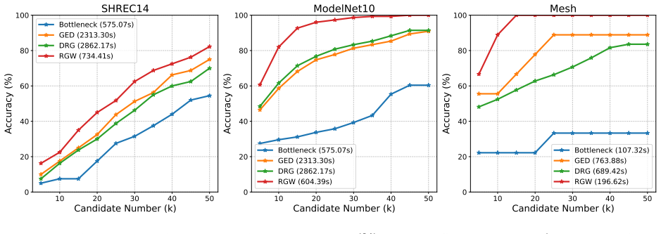
- On the three datasets tested, $\mathrm{RGW}_p$ achieves higher $k$-NN accuracy than bottleneck distance, graph edit distance, and decorated Reeb graphs, with running times comparable to the fastest alternatives.
- Ablation experiments indicate both proposed components contribute: replacing the symmetric Reeb radius or the persistence-image measure with standard alternatives lowers classification accuracy, sometimes substantially.
Reading between the lines
- A testable consequence not pursued in the paper: add controlled noise to a scalar field, compute $\mathrm{RGW}_p$ before and after, and check that the distance grows at most like $\|f-g\|_\infty^{1/p}$; this would directly probe the sharpness of Theorem 5.
- The proof's reliance on a node bijection under perturbation suggests the theorem is most at risk when a persistence pair crosses the diagonal, so an extension would need to handle features that appear or disappear; in that regime the total-variation bound may degrade even if the persistence diagrams are close.
- The same two-component construction could be transferred to Reeb spaces or mapper graphs, since the argument only uses a metric on the quotient space and a stable measure on its nodes.
- Because the experiments use approximate optimal-transport solvers, the practical distance is an approximation of $\mathrm{RGW}_p$; an implicit open question is whether the stability constant $C_1$ can absorb solver error in a way that preserves the theoretical guarantee.
Editorial analysis
A structured set of objections, weighed in public.
Referee Report
Summary. The paper proposes RGWp, a Gromov-Wasserstein distance between Reeb graphs equipped with a symmetrized Reeb radius and a probability measure derived from persistence images of extended persistence diagrams. It claims an L-infinity stability theorem (Theorem 5) bounding RGWp by C1||f-g||_infty^{1/p} + C2 eps^{1/p}, and reports k-NN classification experiments on ModelNet10, SHREC14, and Mesh, with a public implementation.
Significance. The combination of a symmetric Reeb radius and persistence-image weighting is conceptually appealing, and the empirical comparison, ablation study, and hyperparameter sensitivity analysis are useful and clearly reported. If the stability theorem were fully proved, the paper would give an L-infinity stability guarantee for a GW-based Reeb graph distance, which would be a significant contribution. The authors also release source code and describe their experimental setup in sufficient detail. However, the central theoretical claim is not established by the argument as written, because the measure-stability proof rests on an unproven and generally false structural assumption.
major comments (4)
- [Appendix B.3, Theorem 4, Step 3] The proof assumes 'that for sufficiently small ||f-g||_infty, the structural stability of the Reeb graphs ensures a meaningful correspondence (e.g., a bijection gamma ...) between the sets of significant vertices.' This is not a harmless technical assumption: it is a stability statement about the node sets of Reeb graphs of exactly the kind the paper claims to prove, and no proof or reference is supplied. Moreover, the statement is false in this generality: a local extremum pair of small persistence can annihilate under an arbitrarily small L-infinity perturbation, removing two endpoints of persistence intervals from the Reeb graph, so no bijection between the sets of nodes carrying nonzero PI contribution exists. Since the Total Variation bound in Theorem 4 is obtained by summing |nu_Rf(v) - nu_Rg(gamma(v))| over this assumed bijection, and since Theorem 5 (Appendix B.4, Step 2) invokes that TV bound as eta_TV, the main stability theorem does not follow from the proof as written.
- [Appendix B.1, Theorem 2, Eq. (8)] After bounding the functional-variation difference rho_f(x,x') - rho_g(y,y') in the underlying spaces, the proof says 'Assuming this connection allows us to apply Equation (8) appropriately' and equates the Reeb-graph path-based radii rho_f([x],[x']) with the underlying-space quantities rho_f(x,x'). This is a nontrivial quotient-space statement: a path in the underlying space projects to a path in the Reeb graph, but the infimum over Reeb-graph paths could in principle be smaller, and the reverse implication requires an argument or a citation. The gap affects Theorem 3 and hence the delta_GH term in Theorem 5.
- [Appendix B.3, Theorem 4, Step 2] The bound W1(D(f),D(g)) <= N_cells * ||f-g||_infty is asserted for a space 'decomposable into N cells' or under 'suitable discretization assumptions', but Theorem 4 is stated for a compact topological space, and no finite-cell structure or uniform bound on the number of critical points is part of the hypotheses. Even when f and g are Morse on a compact manifold, the number of features is finite for each pair but not uniformly bounded as g approaches f, so the constant M in the conclusion is not shown to exist uniformly in the perturbation. The proof therefore does not establish the claimed Total Variation stability.
- [Sections 3.1 and Appendix B.4, Definitions 7 and 14] Definition 7 defines RGWp as a sum over the finite node sets V_Rf and V_Rg, and Definition 9 produces an atomic measure on endpoints of persistence intervals, while Theorems 3 and 5 use d_GH and d_GP for the full Reeb graphs (Rf,d_Rf). The paper never specifies how the finite-support measure is coupled with the continuum of the Reeb graph as a metric measure space, and the bound d_GP <= max(delta_GH, eta_TV) in Appendix B.4 Step 3 is asserted as a 'standard result' without a precise statement. This is a second obstruction in the passage from the metric and measure stabilities to the final RGWp bound.
minor comments (4)
- [Section 3.2, Proposition 1] Proposition 1 is described both as a 'metric' and as a 'quasi-metric'; since a quasi-metric usually drops symmetry, the two terms are contradictory and should be reconciled.
- [Section 6.2, Figure 8] The ModelNet10 panel reports the same Bottleneck runtime (575.07s) as the SHREC14 panel; please verify whether this is a typo, since the text describes Bottleneck as the fastest method.
- [Section 6.1] The experiments use Mapper graphs rather than exact Reeb graphs, but the relation between the stability theory (which concerns Reeb graphs) and the objects used in the experiments is not discussed.
- [Appendix B.4, Step 3] The inequality d_GP <= max(delta_GH, eta_TV) is attributed to Memoli [27] without a specific lemma or claim; please cite the exact statement, as this is a load-bearing step of the proof.
Circularity Check
Theorem 4's proof assumes a node bijection under perturbation—the structural stability at issue—so the measure-stability bound and final RGWp stability reduce to an unproved assumption.
-
other
[Section 4.2 proof sketch, Step 3; Appendix B.3, Step 3 (proof of Theorem 4)]
"Assuming structural stability of the Reeb graphs under small perturbations of the scalar field (which implies a consistent mapping or bijection γ : VRf → VRg between the sets of significant nodes), we then bound the difference in contributions... / We assume that for sufficiently small ∥f − g∥∞, the structural stability of the Reeb graphs ensures a meaningful correspondence (e.g., a bijection γ : V′ Rf → V′ Rg ) between the respective sets of significant vertices."
The theorem to be proved is d_TV(ν_Rf, ν_Rg) ≤ M∥f−g∥∞, a stability statement for the PI-based measure under L∞ perturbation. In Step 3 the proof assumes, without proof, that small L∞ perturbations give a bijection γ between significant Reeb-graph vertices. That is itself a structural-stability assertion about the node sets on which ν is supported—the same phenomenon the theorem is meant to establish. Low-persistence features can be created or cancelled by arbitrarily small perturbations, so such a bijection is not guaranteed; no threshold or proof is supplied. The subsequent bounds on |contrib_f(v) − contrib_g(γ(v))| and on Z_f−Z_g all depend on this assumed γ, so d_TV ≤ M∥f−g∥∞ is conditional on an unproved stability result.
full rationale
The metric-component stability (Theorems 2–3) is not circular: it relies on the external correspondence/GH framework of Curry et al. and the identity correspondence, plus the stated (L,ε)-connectivity. The PI stability (Adams et al.) and W1 bounds cited for persistence diagrams are also external and independent. The load-bearing problem is in the measure-stability proof (Theorem 4 / Appendix B.3): the proof explicitly assumes a bijection between significant Reeb-graph vertices under small perturbation, i.e., it assumes the structural stability of the very objects whose stability it is proving. Because low-persistence features can annihilate or appear under arbitrarily small L∞ changes, that bijection is not a consequence of the stated Morse-Smale assumptions and is never established. The final RGWp bound (Theorem 5) imports this unproved TV bound, so the central 'small input change ⇒ small RGWp change' claim is only as solid as the assumed structural stability. This is partial circularity (score 6): the derivation does not simply rename a known result, and the metric part is independent, but a core stability prediction reduces to an unproved stability assumption. No self-citation issues were found.
Assumptions & free parameters
free parameters (3)
- PI bandwidth σ =
0.05 (SHREC14), 2 (ModelNet10), 0.5 (Mesh)
- PI resolution N =
10 for all datasets
- Weighting power wp =
2 (SHREC14), 0.1 (ModelNet10), 1 (Mesh)
assumptions (5)
- domain assumption (L, ε)-connectivity of scalar fields (Definition 12)
- domain assumption Morse-Smale / generic Reeb graph regularity
- ad hoc to paper Structural stability of Reeb graph node sets under perturbation
- ad hoc to paper Uniform lower bound on normalization factors and upper bounds on contributions
- standard math Bound dGP ≤ max(δ_GH, η_TV) for metric measure spaces
Cite this review
Pith. "Pith review of A Stable and Theoretically Grounded Gromov-Wasserstein Distance for Reeb Graph Comparison using Persistence Images." pith.science (2026). https://pith.science/paper/5LMU243E
@misc{pith2026250701171,
  author       = {Pith},
  title        = {Pith review of: A Stable and Theoretically Grounded Gromov-Wasserstein Distance for Reeb Graph Comparison using Persistence Images},
  year         = {2026},
  howpublished = {\url{https://pith.science/paper/5LMU243E}},
  note         = {Machine review of arXiv:2507.01171}
}
read the original abstract
Reeb graphs are a fundamental structure for analyzing the topological and geometric properties of scalar fields. Comparing Reeb graphs is crucial for advancing research in this domain, yet existing metrics are often computationally prohibitive or fail to capture essential topological features effectively. In this paper, we explore the application of the Gromov-Wasserstein distance, a versatile metric for comparing metric measure spaces, to Reeb graphs. We propose a framework integrating a symmetric variant of the Reeb radius for robust geometric comparison, and a novel probabilistic weighting scheme based on Persistence Images derived from extended persistence diagrams to effectively incorporate topological significance. A key contribution of this work is the rigorous theoretical proof of the stability of our proposed Reeb Gromov-Wasserstein distance with respect to perturbations in the underlying scalar fields. This ensures that small changes in the input data lead to small changes in the computed distance between Reeb graphs, a critical property for reliable analysis. We demonstrate the advantages of our approach, including its enhanced ability to capture topological features and its proven stability, through comparisons with other alternatives on several datasets, showcasing its practical utility and theoretical soundness.
Figures


Figures from the paper (6 more)



Reference graph
Works this paper leans on
-
[1]
An exact graph edit distance algorithm for solving pattern recognition problems
Zeina Abu-Aisheh, Romain Raveaux, Jean-Yves Ramel, and Patrick Martineau. An exact graph edit distance algorithm for solving pattern recognition problems. In 4th International 24 Conference on Pattern Recognition Applications and Methods 2015 , 2015
work page 2015
-
[2]
Persistence images: A stable vector representation of persistent homology
Henry Adams, Tegan Emerson, Michael Kirby, Rachel Neville, Chris Peterson, Patrick Ship- man, Sofya Chepushtanova, Eric Hanson, Francis Motta, and Lori Ziegelmeier. Persistence images: A stable vector representation of persistent homology. Journal of Machine Learning Research, 18(8):1–35, 2017
work page 2017
-
[3]
Extreme elevation on a 2-manifold
Pankaj K Agarwal, Herbert Edelsbrunner, John Harer, and Yusu Wang. Extreme elevation on a 2-manifold. In Proceedings of the twentieth annual symposium on Computational geometry , pages 357–365, 2004
work page 2004
-
[4]
Enrique G Alvarado, Robin Belton, Kang-Ju Lee, Sourabh Palande, Sarah Percival, Em- ilie Purvine, and Sarah Tymochko. Any graph is a mapper graph. arXiv preprint arXiv:2408.11180, 2024
arXiv 2024
-
[5]
Measuring distance between reeb graphs
Ulrich Bauer, Xiaoyin Ge, and Yusu Wang. Measuring distance between reeb graphs. In Proceedings of the thirtieth annual symposium on Computational geometry , pages 464–473, 2014
work page 2014
-
[6]
The Reeb graph edit distance is universal
Ulrich Bauer, Claudia Landi, and Facundo M´ emoli. The Reeb graph edit distance is universal. Foundations of Computational Mathematics , pages 1–24, 2021
work page 2021
-
[7]
Stability of higher-dimensional interval decomposable persistence modules
H ˚ avard Bakke Bjerkevik. Stability of higher-dimensional interval decomposable persistence modules. arXiv preprint arXiv:1609.02086 , 2016
work page Pith review arXiv 2016
-
[8]
Reeb graph metrics from the ground up
Brian Bollen, Erin Chambers, Joshua A Levine, and Elizabeth Munch. Reeb graph metrics from the ground up. arXiv preprint arXiv:2110.05631 , 2021
arXiv 2021
Show all 52 references
-
[9]
A Course in Metric Geometry , volume 33 of Graduate Studies in Mathematics
Dmitri Burago, Yuri Burago, and Sergei Ivanov. A Course in Metric Geometry , volume 33 of Graduate Studies in Mathematics . American Mathematical Society, Providence, RI, 2001
2001
-
[10]
Extending persistence using Poincar´ e and Lefschetz duality
David Cohen-Steiner, Herbert Edelsbrunner, and John Harer. Extending persistence using Poincar´ e and Lefschetz duality. Foundations of Computational Mathematics , 9(1):79–103, 2009
2009
-
[11]
Topologically attributed graphs for shape discrimination
Justin Curry, Washington Mio, Tom Needham, Osman Berat Okutan, and Florian Russold. Topologically attributed graphs for shape discrimination. In Topological, Algebraic and Geo- metric Learning Workshops 2023 , pages 87–101. PMLR, 2023
2023
-
[12]
Stability and approximations for decorated Reeb spaces
Justin Curry, Washington Mio, Tom Needham, Osman Berat Okutan, and Florian Russold. Stability and approximations for decorated Reeb spaces. In 40th International Symposium on Computational Geometry (SoCG 2024) . Schloss Dagstuhl–Leibniz-Zentrum f¨ ur Informatik, 2024
2024
-
[13]
Categorified Reeb graphs
Vin De Silva, Elizabeth Munch, and Amit Patel. Categorified Reeb graphs. Discrete & Computational Geometry, 55(4):854–906, 2016
2016
-
[14]
Dey and Yusu Wang
Tamal K. Dey and Yusu Wang. Computational Topology for Data Analysis . Cambridge Uni- versity Press, Cambridge, England, 2022. 25
2022
-
[15]
The edit distance for Reeb graphs of surfaces
Barbara Di Fabio and Claudia Landi. The edit distance for Reeb graphs of surfaces. Discrete & Computational Geometry , 55:423–461, 2016
2016
-
[16]
Complexity fusion for indexing Reeb digraphs
Francisco Escolano, Edwin R Hancock, and Silvia Biasotti. Complexity fusion for indexing Reeb digraphs. In International Conference on Computer Analysis of Images and Patterns , pages 120–127. Springer, 2013
2013
-
[17]
Pot: Python optimal transport
R´ emi Flamary, Nicolas Courty, Alexandre Gramfort, Mokhtar Z Alaya, Aur´ elie Boisbunon, Stanislas Chambon, Laetitia Chapel, Adrien Corenflos, Kilian Fatras, Nemo Fournier, et al. Pot: Python optimal transport. Journal of Machine Learning Research , 22(78):1–8, 2021
2021
-
[18]
Data skeletonization via Reeb graphs
Xiaoyin Ge, Issam Safa, Mikhail Belkin, and Yusu Wang. Data skeletonization via Reeb graphs. Advances in neural information processing systems , 24, 2011
2011
-
[19]
Shrec’14 track: Shape retrieval of non-rigid 3d human models, 2014
Afzal A Godil and Chunyuan Li. Shrec’14 track: Shape retrieval of non-rigid 3d human models, 2014
2014
-
[20]
Exploring network structure, dynamics, and function using networkx
Aric Hagberg, Pieter J Swart, and Daniel A Schult. Exploring network structure, dynamics, and function using networkx. Technical report, Los Alamos National Laboratory (LANL), Los Alamos, NM (United States), 2008
2008
-
[21]
Topology match- ing for fully automatic similarity estimation of 3d shapes
Masaki Hilaga, Yoshihisa Shinagawa, Taku Kohmura, and Tosiyasu L Kunii. Topology match- ing for fully automatic similarity estimation of 3d shapes. In Proceedings of the 28th annual conference on Computer graphics and interactive techniques , pages 203–212, 2001
2001
-
[22]
Scalable optimal transport methods in machine learning: A contemporary survey
Abdelwahed Khamis, Russell Tsuchida, Mohamed Tarek, Vivien Rolland, and Lars Peters- son. Scalable optimal transport methods in machine learning: A contemporary survey. IEEE Transactions on Pattern Analysis and Machine Intelligence , 2024
2024
-
[23]
Shapevis: High- dimensional data visualization at scale
Nupur Kumari, Akash Rupela, Piyush Gupta, and Balaji Krishnamurthy. Shapevis: High- dimensional data visualization at scale. In Proceedings of The Web Conference 2020 , pages 2920–2926, 2020
2020
-
[24]
Comparing Morse complexes using optimal transport: An experimental study
Mingzhe Li, Carson Storm, Austin Yang Li, Tom Needham, and Bei Wang. Comparing Morse complexes using optimal transport: An experimental study. In 2023 IEEE Visualization and Visual Analytics (VIS) , pages 41–45. IEEE, 2023
2023
-
[25]
Flexible and probabilistic topology tracking with partial optimal transport
Mingzhe Li, Xinyuan Yan, Lin Yan, Tom Needham, and Bei Wang. Flexible and probabilistic topology tracking with partial optimal transport. arXiv preprint arXiv:2302.02895 , 2023
2023 arXiv
-
[26]
The gudhi library: Simplicial complexes and persistent homology
Cl´ ement Maria, Jean-Daniel Boissonnat, Marc Glisse, and Mariette Yvinec. The gudhi library: Simplicial complexes and persistent homology. In Mathematical Software–ICMS 2014: 4th International Congress, Seoul, South Korea, August 5-9, 2014. Proceedings 4 , pages 167–174. Spri...
2014
-
[27]
Gromov–Wasserstein distances and the metric approach to object matching
Facundo M´ emoli. Gromov–Wasserstein distances and the metric approach to object matching. Foundations of computational mathematics , 11:417–487, 2011
2011
-
[28]
Morse Theory
John Milnor. Morse Theory. Princeton University Press, Princeton, NJ, 1963. 26
1963
-
[29]
Recent advances in optimal transport for machine learning
Eduardo Fernandes Montesuma, Fred Maurice Ngol` e Mboula, and Antoine Souloumiac. Recent advances in optimal transport for machine learning. IEEE Transactions on Pattern Analysis and Machine Intelligence , 2024
2024
-
[30]
Persistence theory: from quiver representations to data analysis , volume 209 of Mathematical Surveys and Monographs
Steve Y Oudot. Persistence theory: from quiver representations to data analysis , volume 209 of Mathematical Surveys and Monographs . American Mathematical Soc., Providence, Rhode Island, 2017
2017
-
[31]
Computational optimal transport: With applications to data science
Gabriel Peyr´ e, Marco Cuturi, et al. Computational optimal transport: With applications to data science. Foundations and Trends® in Machine Learning , 11(5-6):355–607, 2019
2019
-
[32]
Topological shape matching using multi- dimensional reeb graphs
Yashwanth Ramamurthi and Amit Chattopadhyay. Topological shape matching using multi- dimensional reeb graphs. In Proceedings of the Thirteenth Indian Conference on Computer Vision, Graphics and Image Processing , pages 1–10, 2022
2022
-
[33]
The Laplacian on a Riemannian Manifold: An Introduction to Analysis on Manifolds
Steven Rosenberg. The Laplacian on a Riemannian Manifold: An Introduction to Analysis on Manifolds . London Mathematical Society Student Texts. Cambridge University Press, Cambridge, 1997
1997
-
[34]
Topological methods for the analysis of high dimensional data sets and 3d object recognition
Gurjeet Singh, Facundo M´ emoli, Gunnar E Carlsson, et al. Topological methods for the analysis of high dimensional data sets and 3d object recognition. PBG@ Eurographics, 2: 091–100, 2007
2007
-
[35]
Wasserstein stability for persistence diagrams
Primoz Skraba and Katharine Turner. Wasserstein stability for persistence diagrams. arXiv preprint arXiv:2006.16824, 2020
2006 arXiv
-
[36]
Entropic metric alignment for correspondence problems
Justin Solomon, Gabriel Peyr´ e, Vladimir G Kim, and Suvrit Sra. Entropic metric alignment for correspondence problems. ACM Transactions on Graphics (ToG) , 35(4):1–13, 2016
2016
-
[37]
Mesh data from deformation transfer for triangle meshes, 2004
R W Sumner and J Po-povic. Mesh data from deformation transfer for triangle meshes, 2004
2004
-
[38]
3d mesh skeleton extraction using topological and geometrical analyses
Julien Tierny, Jean-Philippe Vandeborre, and Mohamed Daoudi. 3d mesh skeleton extraction using topological and geometrical analyses. In 14th Pacific Conference on Computer Graphics and Applications (Pacific Graphics 2006) , page s1poster, 2006
2006
-
[39]
Ripser.py: A lean persistent homology library for python
Christopher Tralie, Nathaniel Saul, and Rann Bar-On. Ripser.py: A lean persistent homology library for python. The Journal of Open Source Software , 3(29):925, Sep 2018. doi: 10.21105/ joss.00925. URL https://doi.org/10.21105/joss.00925
2018 doi
-
[40]
Measure theo- retic Reeb graphs and Reeb spaces
Qingsong Wang, Guanqun Ma, Raghavendra Sridharamurthy, and Bei Wang. Measure theo- retic Reeb graphs and Reeb spaces. arXiv preprint arXiv:2401.06748 , 2024
2024 arXiv
-
[41]
3d shapenets: A deep representation for volumetric shapes
Zhirong Wu, Shuran Song, Aditya Khosla, Fisher Yu, Linguang Zhang, Xiaoou Tang, and Jianxiong Xiao. 3d shapenets: A deep representation for volumetric shapes. In Proceedings of the IEEE conference on computer vision and pattern recognition , pages 1912–1920, 2015
1912
-
[42]
Gromov-wasserstein learning for graph matching and node embedding
Hongteng Xu, Dixin Luo, Hongyuan Zha, and Lawrence Carin Duke. Gromov-wasserstein learning for graph matching and node embedding. In International conference on machine learning, pages 6932–6941. PMLR, 2019. 27
2019
-
[43]
Scalar field comparison with topological descriptors: Properties and applications for scientific visualization
Lin Yan, Talha Bin Masood, Raghavendra Sridharamurthy, Farhan Rasheed, Vijay Natarajan, Ingrid Hotz, and Bei Wang. Scalar field comparison with topological descriptors: Properties and applications for scientific visualization. In Computer Graphics Forum , volume 40, pages 599–...
2021
-
[44]
Since abso- lute values are inherently non-negative, their supremum over any path is also non-negative
Non-negativity: The Reeb radius ρf (x, y) is defined as an infimum of suprema of absolute differences of function values, specifically sup t∈[0,1] | ¯f (x) − ¯f (γ(t))| for paths γ. Since abso- lute values are inherently non-negative, their supremum over any path is also non-n...
-
[45]
For this path, ¯f (γ(t)) = ¯f (x) for all t, so sup t∈[0,1] | ¯f (x) − ¯f (γ(t))| = 0
Identity of Indiscernibles: If x = y, then the path γ from x to x can be the trivial path consisting only of the node x. For this path, ¯f (γ(t)) = ¯f (x) for all t, so sup t∈[0,1] | ¯f (x) − ¯f (γ(t))| = 0. Thus, ρf (x, x) = 0. This implies dRf (x, x) = 1 2 (ρf (x, x) + ρf (x...
-
[46]
Hence, dRf is symmetric
Symmetry: This property follows directly and trivially from the definition of dRf : dRf (x, y) = 1 2 (ρf (x, y) + ρf (y, x)) = 1 2 (ρf (y, x) + ρf (x, y)) = dRf (y, x). Hence, dRf is symmetric
-
[47]
The critical preliminary step is to establish the triangle inequality for the (potentially asymmetric) Reeb radius ρf itself: ρf (x, z) ≤ ρf (x, y) + ρf (y, z)
T riangle Inequality: We need to show that dRf (x, z) ≤ dRf (x, y) + dRf (y, z). The critical preliminary step is to establish the triangle inequality for the (potentially asymmetric) Reeb radius ρf itself: ρf (x, z) ≤ ρf (x, y) + ρf (y, z). (5) To prove Equation (5), let x, y...
-
[48]
34 Next, we consider the normalization factorsZf = P u∈V ′ Rf contribf (u) and Zg = P u∈V ′ Rg contribg(u)
is a new constant. 34 Next, we consider the normalization factorsZf = P u∈V ′ Rf contribf (u) and Zg = P u∈V ′ Rg contribg(u). The difference is bounded by: |Zf − Zg| ≤ X v∈V ′ Rf |contribf (v) − contribg(γ(v))| ≤VN C′∥f − g∥∞. Assuming Zf , Zg ≥ mZ > 0 (i.e., the total contri...
-
[49]
We denote this upper bound as δGH := (L + 1)∥f − g∥∞ + ϵ
Step 1: Bounding Metric Component Closeness ( δGH ) From Theorem 3, we have established that the Gromov-Hausdorff distance between the metric structures of the Reeb graphs, (Rf , dRf ) and ( Rg, dRg ), is bounded by: dGH((Rf , dRf ), (Rg, dRg )) ≤ (L + 1)∥f − g∥∞ + ϵ. We denot...
-
[50]
We denote this upper bound as ηT V:= M ∥f − g∥∞
Step 2: Bounding Measure Component Closeness ( ηT V) From Theorem 4, the Total Variation distance between the probability measures νRf and νRg on the Reeb graph nodes is bounded by: dT V(νRf , νRg ) ≤ M ∥f − g∥∞. We denote this upper bound as ηT V:= M ∥f − g∥∞. (The statement ...
-
[51]
Standard results in the theory of metric measure spaces (e.g., arguments found in M´ emoli [27]) provide a bound of the form: dGP(R∗ f , R∗ g) ≤ max(δGH , ηT V)
Step 3: Bounding the Gromov-Prokhorov Distance ( dGP) The Gromov-Prokhorov distance dGP(R∗ f , R∗ g) between the two metric measure spaces is controlled by both the geo- metric dissimilarity (related to δGH ) and the measure discrepancy (related to ηT V). Standard results in t...
-
[52]
Step 4: Deriving the Final Bound onRGWp We now substitute this bound fordGP(R∗ f , R∗ g) into M´ emoli’s inequality (Equation (12)): RGWp(R∗ f , R∗ g) ≤ (K0∥f − g∥∞ + ϵ)1/p (Dp max + 1)1/p. Using the standard inequality ( a + b)k ≤ ak + bk for a, b≥ 0 and 0 < k≤ 1 (here k = 1/...
Reviewed August 6, 2026 · model on record in the stance chip above.
Discussion (0). Continue with ORCID to comment.