REVIEW 3 major objections 5 minor 1 cited by
The Lockman-SpReSO project. Spectroscopic analysis of Type 1 AGN
T0 review · 3 major / 5 minor · reviewed 2026-08-06 · deepseek-v4-flash
Pith's one-line read FIR/X-ray-selected quasars follow the same quasar main sequence
desk verdict Solid, useful sample paper with genuinely new measurements; the QMS population counts are internally inconsistent and the UV classification caveat needs a sharper statement, but the core is publishable after revision. read the letter →
The pith
A machine-rendered reading of the paper's core claim, the machinery that carries it, and where it could break.
The reading
What carries the argument
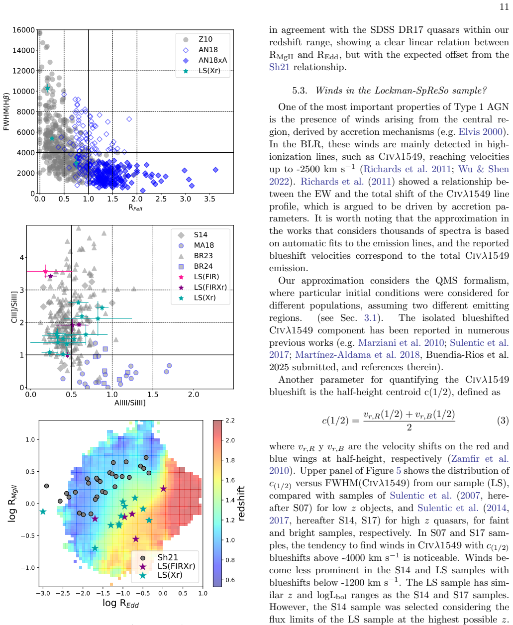
The load-bearing machinery is the Quasar Main Sequence (QMS) phenomenology: an optical classification scheme, originally defined by H$\beta$ FWHM and Fe II strength, that sorts Type 1 AGN into Population A (FWHM below 4000 km s$^{-1}$, Lorentzian profiles, stronger Fe II) and Population B (Gaussian profiles, weak Fe II). To apply it to UV-only spectra, the paper uses two substitutes: a line-profile decomposition that separates a virialized broad component from blueshifted wind or very broad redshifted components, and a UV line-ratio diagram (C III]/Al III against Al III/Si III]) that places objects without H$\beta$ on the same sequence. Black hole masses are computed from Equation (1) using four single-epoch virial calibrators: VP06 for H$\beta$, TN12 for Mg II, BR23 for Al III, and M19 for C IV, each applied to the isolated broad component.
What would settle it
Obtain rest-frame optical spectra covering H$\beta$ and Fe II for the objects classified as Population B from UV data alone; if a substantial fraction show FWHM(H$\beta$) below 4000 km s$^{-1}$ and strong Fe II, placing them in Population A or the xA domain, then the claimed Population-B dominance and absence of extreme accretors would not hold.
Extended reading notes
Core claim
The central claim is that a spectroscopically faint, far-infrared and X-ray selected sample of 30 Type 1 AGN reproduces the correlations used to organize optically selected quasars. On the paper's own terms: the sample spans $\log L_{\rm bol} = 44.85$\textendash$47.87$, $\log M_{\rm BH} = 7.59$\textendash$9.80$, and $\log R_{\rm Edd} = -1.70$ to $+0.56$; 25 objects fall in Population B and 5 in Population A, with none in the extreme-accretor (xA) domain; C IV half-height centroids $c(1/2)$ are between $941$ and $-1587$ km s$^{-1}$; the Baldwin effect slope is $-0.23 \pm 0.03$; and the Eddington-ratio/FWHM anticorrelation is $\log R_{\rm Edd} = -0.17\,{\rm FWHM}_{1000}({\rm BC}) + 0.27$ with $r_p = -0.7$. The authors also recover the $R_{\rm MgII}$\textendash$R_{\rm Edd}$ relation seen in SDSS DR17 and find no variability between Lockman-SpReSO and SDSS spectra of the same objects.
Load-bearing premise
The load-bearing premise is that the Population A/B axis, defined optically by H$\beta$ FWHM and Fe II strength, can be recovered from UV-only spectra through broad-component profile shape (Lorentzian versus Gaussian), the 4000 km s$^{-1}$ FWHM boundary, and the C III]/Al III versus Al III/Si III] diagram, with single-epoch virial calibrators for Mg II, Al III, and C IV that are assumed to trace the same virialized gas at high redshift.
Editorial extensions
If this is right
- Faint FIR/X-ray-selected Type 1 AGN are not preferentially extreme accretors; none of the 30 objects reaches the xA domain.
- Modest C IV blueshifts, with $c(1/2)$ between 941 and $-1587$ km s$^{-1}$, imply that outflow activity in this sample resembles that of optically selected samples of similar redshift and absolute magnitude.
- The Baldwin effect slope of $-0.23 \pm 0.03$ extends the C IV equivalent-width versus luminosity anti-correlation to a FIR/X-ray-selected population, supporting a common origin tied to the Eddington ratio.
- The recovered $R_{\rm Edd}$\textendash FWHM(BC) anticorrelation indicates that single-epoch spectral fits can track the accretion rate in faint, high-redshift samples.
- Agreement between Lockman-SpReSO and SDSS spectra of the same objects suggests that single-epoch classifications are stable within errors over the sampled time baseline.
Reading between the lines
- If FIR and X-ray selection does not shift main-sequence demographics, then infrared-selected surveys can serve as relatively unbiased tracers of supermassive black hole accretion at high redshift; this is an extension the paper only hints at.
- The complete absence of extreme accretors among 30 objects could be a small-sample effect or a consequence of FIR selection preferring lower-Eddington, dustier systems; a sample of order 100 objects would distinguish these alternatives.
- The paper documents a redshift-dependent family of $R_{\rm MgII}$\textendash$R_{\rm Edd}$ relations without modeling it; a testable extension is to recalibrate Mg II Eddington ratios as a function of redshift using the SDSS DR17 data it compiled.
- Rest-frame optical spectroscopy of the high-redshift UV-classified objects would directly test whether Lorentzian-profile Population A assignments at $z>2$ agree with H$\beta$-based classifications.
Editorial analysis
A structured set of objections, weighed in public.
Referee Report
Summary. This paper presents a spectroscopic analysis of 30 Type 1 AGN selected from the Lockman-SpReSO survey in the FIR and X-ray, covering redshifts 0.46 < z < 4.97 and faint B-band magnitudes. The authors fit the optical-UV spectra using the Quasar Main Sequence (QMS) methodology, deblending Lyα, Si iv, C iv, the 1900 Å blend, Mg ii, and Hβ, and derive bolometric luminosities, virial black hole masses, and Eddington ratios. They assign the objects to QMS Populations A and B, find no extreme accretors, measure C iv half-height centroid shifts as a wind diagnostic, recover the Baldwin effect with slope -0.23 ± 0.03, compare 12 objects with SDSS DR17 spectra to look for variability, and perform a Galactic extinction check. The central claim is that this faint, FIR/X-ray-selected sample follows the same quasar main sequence relations as optically selected samples, with a predominantly Population B composition.
Significance. If the classification is robust, this is a valuable first systematic QMS analysis of a faint FIR/X-ray-selected Type 1 AGN sample, extending the QMS framework to the UV at z ~ 2-5 and showing that selection at long wavelengths does not produce obvious differences in the optical-UV spectroscopic eigenvector plane. The paper has several strengths: the fitting procedure is described in unusual detail, errors are propagated to the derived quantities, the authors explicitly acknowledge that the R_Edd-FWHM anti-correlation is partly constructed from the FWHM-based mass estimator, and the SDSS DR17 comparison is a good-faith cross-check. However, the headline population statistics rest on UV-only proxies for the majority of the sample, and the reported population counts are internally inconsistent across the abstract, Section 5.1, and Section 6. These issues are fixable in revision but currently prevent the paper's main quantitative claims from being accepted as they stand.
major comments (3)
- [§5.1; §3.1] The claim that 25 of 30 objects are Population B and none is an extreme accretor rests heavily on UV-only proxies, and for nine objects the proxy is not independent of the population definition. Section 3.1 sets the profile choice by FWHM: Lorentzian for FWHM < 4000 km/s and Gaussian for FWHM > 4000 km/s, while Section 5.1 assigns four C iv-only objects to Population A because their profile is Lorentzian and one to Population B because it is Gaussian. Since the A/B boundary is itself FWHM(Hβ) = 4000 km/s, these assignments merely restate the FWHM that also enters the virial mass estimate, rather than providing an independent UV-photoionization test. For the 18 objects placed via the C iii]/Al iii versus Al iii/Si iii] diagram the method is more defensible, but the three objects at the Population A boundary and the reliance on Marziani & Sulentic (2014) calibrators at z ~ 2-5 need a sensitivity test (e.g., FWHM-only classification, bootstrap reclassification, or stacked spectra) before the Population B dominance can be considered robust.
- [Abstract; §5.1; §6] The population counts are internally inconsistent. The abstract reports 18 high-z Population B, three low-z objects (A2, B1, B1+), and "the remaining eight are candidates to be Pop. B and one Pop. A object", which sums to 30 but implies a different B/A split than the text. Section 5.1's detailed enumeration gives 18 (1900-Å blend, Pop B) + 3 (Mg ii, Pop B) + 1 (C iv Gaussian, Pop B) = 22 high-z B and 4 + 1 = 5 high-z A, before adding the three low-z objects, yet ends with "25 Pop. B and 5 Pop. A objects". Section 6 states 23 high-z B and 4 high-z A, which is yet a third distribution. Please reconcile these counts and make the per-object population table available so that the summary numbers can be reproduced.
- [§5.1; Fig. 4] The claim that none of the 18 objects in the UV diagram lies in the xA domain cannot be checked from the paper, because the measured C iii]/Al iii and Al iii/Si iii] ratios and their errors are not reported. Please add a table (or machine-readable column) with these ratios, the adopted profile/FWHM for each object, and the resulting population and sub-population, so the boundary placement in Fig. 4 is transparent.
minor comments (5)
- [Abstract] The redshift range in the abstract is printed as "0.33 > z > 4.97", which has the inequality signs reversed and disagrees with the value 0.46 < z < 4.97 given in §2.1 and Table 1; please correct it.
- [§5.4] The phrase "with a p-value of -0.67" after Eq. (4) is presumably the Pearson correlation coefficient r, not a p-value; please rename it accordingly.
- [§5.5] The number of SDSS DR17 matches is inconsistent: Table 1 lists 12 objects and the abstract says 12, but §5.5 says "We found 10 of these"; please clarify how many spectra actually entered the variability comparison and why any were excluded.
- [§4; Table 3] Table 3 reports only an average FWHM(BC) for each object, but Eq. (1) is evaluated separately for Hβ, Mg ii, Al iii, and C iv with different calibrators; reporting the line-specific FWHM and luminosity used for each mass estimate would improve reproducibility.
- [§6] The summary states the Mg ii subsample as "0.462 > z > 1.956", again with inverted inequality signs; the intended range is 0.462 < z < 1.956.
Circularity Check
The REdd-FWHM anti-correlation (Eq. 2) is partly built into the virial MBH estimator, but the paper explicitly acknowledges this and anchors it with an independent X-ray-based relation, while the central QMS and population claims rest on external calibrations.
-
self definitional
[Section 4, Eq. (2) and following paragraph; Fig. 3 lower panel]
"We observed a clear trend in the REdd vs. FWHM plot and derived the anti-correlation using the FWHM normalized by 1000 km s−1: logREdd = −0.17 FWHM1000(BC) + 0.27 (2) with a correlation coefficient rp=-0.7. The correlation described above is expected as the MBH that is used to compute REdd uses the FWHM values."
By Eq. (1), log MBH = 2 log(FWHM/1000) + α log(λLλ) + β (plus a constant). Since REdd ≡ Lbol/LEdd and LEdd ∝ MBH, log REdd = log Lbol − log MBH + const, so any object-to-object change in FWHM induces an anti-correlation in log REdd through the estimator itself. The regression slope -0.17 is therefore not an independent empirical discovery; it is a transformation of the input FWHM used to construct MBH. The paper explicitly concedes this ('expected as the MBH ... uses the FWHM values') and mitigates it by citing an X-ray-mass-based relation (Marziani et al. 2001), which is external evidence.
full rationale
The paper is primarily a measurement and classification study. Bolometric luminosities are computed from continuum windows with published bolometric corrections; black hole masses use Eq. (1) with external virial calibrators (VP06, TN12, BR23, M19) that are not fitted to the present sample or to the quantities being reported. The Baldwin effect slope (−0.23 ± 0.03) is an empirical fit to EW(C IV) versus L(1350), a relation that is not forced to this value by the definition of EW alone; the paper compares it to independent literature, so it is not circular. The C IV half-height centroid wind measurements are direct spectral measurements. The Population A/B and xA classifications apply an externally established QMS taxonomy; whether that taxonomy extends reliably to UV-only spectra is a physical assumption and a correctness risk, not a logical circularity. The one genuine circular reduction is Eq. (2): because REdd is computed from MBH, which is itself derived from FWHM via Eq. (1), the observed REdd-FWHM anti-correlation is partly constructed. The authors explicitly label it 'expected' and cite an independent X-ray-based relation (Marziani et al. 2001) as external support. The centrality of this constructed correlation is limited, and the paper's other headline results retain independent empirical content, so the overall circularity score is moderate rather than severe.
Assumptions & free parameters
free parameters (4)
- REdd-FWHM slope =
-0.17
- REdd-FWHM intercept =
0.27
- Baldwin effect slope =
-0.23 ± 0.03
- Baldwin effect intercept =
11.75 ± 0.23
assumptions (5)
- standard math Concordance cosmology with H0=70 km/s/Mpc, Omega_m=0.3, Omega_Lambda=0.7 is assumed for distance and luminosity computations.
- domain assumption The single-epoch virial MBH estimator (Eq. 1) using Hbeta, MgII, AlIII, CIV line widths and continuum luminosities with literature calibrators yields reliable MBH for these high-z faint AGN.
- domain assumption QMS Population A/B classification defined by FWHM(Hbeta)=4000 km/s can be extended to objects without Hbeta using FWHM and line-profile proxies from CIV, MgII, Ly alpha.
- domain assumption The spectral decomposition into virialized broad component, blueshifted wind component, very broad redshifted component, narrow lines with shared kinematics, and FeII templates (Bruhweiler & Verner 2008, Vestergaard & Wilkes 2001) uniquely recovers the physical components.
- domain assumption CIV half-height centroid c(1/2) (Eq. 3) is a valid proxy for wind velocities in the BLR.
Cite this review
Pith. "Pith review of The Lockman-SpReSO project. Spectroscopic analysis of Type 1 AGN." pith.science (2026). https://pith.science/paper/C26IXCED
@misc{pith2026250701952,
  author       = {Pith},
  title        = {Pith review of: The Lockman-SpReSO project. Spectroscopic analysis of Type 1 AGN},
  year         = {2026},
  howpublished = {\url{https://pith.science/paper/C26IXCED}},
  note         = {Machine review of arXiv:2507.01952}
}
read the original abstract
We present the first optical-UV spectral systematic analysis of 30 Type 1 AGN selected in the FIR and X-ray in the Lockman-SpReSO Survey. The sample of faint objects (m_B = 19.6-21.8) covers a large redshift range of 0.33 > z > 4.97 with high S/N (~21 on average). A detailed spectral analysis based on the Quasar Main Sequence phenomenology prescription was applied to deblend the principal optical-UV emitting regions. Our sample spans a bolometric luminosity range of 44.85 < log Lbol < 47.87, absolute B-magnitude -20.46 > M_B > -26.14, BH mass of 7.59 < log MBH < 9.80, and Eddington ratio -1.70 < log REdd < 0.56. The analysis shows that 18 high-z objects correspond to Population B, whereas three low-z fall in Populations A2, B1, and B1+. The remaining eight are candidates to be Pop. B and one Pop. A object. None of them are extreme accretors. We looked for tendencies in our sample and compared them with other samples with different selection criteria. Evidence for winds was explored using CIV1549 line half-height centroid cmed finding wind velocities between 941 and -1587 kms-1. This result is consistent with samples with similar ranges of z and M_B. The Baldwin effect showed a slope of -0.23 pm 0.03 dex consistent with previous studies. Spectra from twelve objects in our sample were found in the Sloan Digital Sky Survey Data Release 17 database. We applied the same methodology to compare them to our spectra, finding no evidence of variability.
Figures


Figures from the paper (2 more)

Forward citations
Cited by 1 Pith paper
-
The Lockman-SpReSO Project: A Deep X-ray Spectral View of a FIR-selected AGN Population
X-ray analysis of 94 FIR-selected AGNs at z=0.07-5 shows rising obscured fraction with redshift, soft excess in 10 sources, and a luminosity-dependent covering factor correlation supporting the receding torus model.
Reference graph
Works this paper leans on
-
[1]
2022, ApJS, 259, 35, doi: 10.3847/1538-4365/ac4414
Abdurro’uf, Accetta, K., Aerts, C., et al. 2022, ApJS, 259, 35, doi: 10.3847/1538-4365/ac4414
-
[2]
Bachev, R., Marziani, P., Sulentic, J. W., et al. 2004, ApJ, 617, 171, doi: 10.1086/425210
-
[3]
Baldwin, J. A. 1977, ApJ, 214, 679, doi: 10.1086/155294
doi:10.1086/155294 1977
-
[4]
Baldwin, J. A., Phillips, M. M., & Terlevich, R. 1981, PASP, 93, 5, doi: 10.1086/130766 Ben ´ ıtez, E., Ibarra-Medel, H., Negrete, C. A., et al. 2023, ApJ, 952, 45, doi: 10.3847/1538-4357/acce3e Ben ´ ıtez, E., Jim´ enez-Bail´ on, E., Negrete, C. A., et al. 2022, MNRAS, 516, 5270, doi: 10.1093/mnras/stac2244
doi:10.1086/130766 1981
-
[6]
2019, A&A, 622, A103, doi: 10.1051/0004-6361/201834156
Boquien, M., Burgarella, D., Roehlly, Y., et al. 2019, A&A, 622, A103, doi: 10.1051/0004-6361/201834156
-
[7]
Boroson, T. A., & Green, R. F. 1992, ApJS, 80, 109, doi: 10.1086/191661
doi:10.1086/191661 1992
-
[8]
2008, ApJ, 675, 83, doi: 10.1086/525557
Bruhweiler, F., & Verner, E. 2008, ApJ, 675, 83, doi: 10.1086/525557
doi:10.1086/525557 2008
-
[9]
2023, A&A, 669, A135, doi: 10.1051/0004-6361/202244177
Dultzin, D. 2023, A&A, 669, A135, doi: 10.1051/0004-6361/202244177
Show all 66 references
-
[10]
A., Clayton, G
Cardelli, J. A., Clayton, G. C., & Mathis, J. S. 1989, ApJ, 345, 245, doi: 10.1086/167900
1989 doi
-
[11]
M., & Lockman, F
Dickey, J. M., & Lockman, F. J. 1990, ARA&A, 28, 215, doi: 10.1146/annurev.aa.28.090190.001243
1990
- [12]
-
[13]
J., Hu, C., Wang, J., et al
Ferland, G. J., Hu, C., Wang, J., et al. 2009, ApJL, 707, L82, doi: 10.1088/0004-637X/707/1/L82
2009 doi
-
[14]
2012, ApJS, 198, 1, doi: 10.1088/0067-0049/198/1/1
Fotopoulou, S., Salvato, M., Hasinger, G., et al. 2012, ApJS, 198, 1, doi: 10.1088/0067-0049/198/1/1
2012 doi
-
[15]
J., Hewett, P
Francis, P. J., Hewett, P. C., Foltz, C. B., et al. 1991, ApJ, 373, 465, doi: 10.1086/170066
1991 doi
-
[16]
A., Marziani, P., et al
Garnica, K., Negrete, C. A., Marziani, P., et al. 2022, A&A, 667, A105, doi: 10.1051/0004-6361/202142837
2022 doi
-
[17]
2016, MNRAS, 462, 966, doi: 10.1093/mnras/stw1605
Ge, X., Bian, W.-H., Jiang, X.-L., Liu, W.-S., & Wang, X.-F. 2016, MNRAS, 462, 966, doi: 10.1093/mnras/stw1605
2016 doi
-
[18]
P., Cepa, J., et al
Gonzalez-Otero, M., Padilla-Torres, C. P., Cepa, J., et al. 2023, A&A, 669, A85, doi: 10.1051/0004-6361/202244480 Gonz´ alez-Otero, M., Cepa, J., Padilla-Torres, C. P., et al. 2024, A&A, 687, A19, doi: 10.1051/0004-6361/202449238 Gr¨ unwald, G., Boller, T., Rakshit, S., et al....
2023 doi
-
[19]
A., Lacerna, I., et al
Ibarra-Medel, H., Negrete, C. A., Lacerna, I., et al. 2025, MNRAS, 536, 752, doi: 10.1093/mnras/stae2623
2025 doi
-
[20]
K., & Ammon, K
Jordi, K., Grebel, E. K., & Ammon, K. 2006, A&A, 460, 339, doi: 10.1051/0004-6361:20066082
2006 doi
-
[21]
2009, A&A, 494, L25, doi: 10.1051/0004-6361:200811415
Juarez, Y., Maiolino, R., Mujica, R., et al. 2009, A&A, 494, L25, doi: 10.1051/0004-6361:200811415
2009 doi
-
[22]
2013, A&A, 549, A100, doi: 10.1051/0004-6361/201219411
Kollatschny, W., & Zetzl, M. 2013, A&A, 549, A100, doi: 10.1051/0004-6361/201219411
2013 doi
-
[23]
N., Hardcastle, M
Kondapally, R., Best, P. N., Hardcastle, M. J., et al. 2021, A&A, 648, A3, doi: 10.1051/0004-6361/202038813 Kovaˇ cevi´ c, J., Popovi´ c, L.ˇC., & Dimitrijevi´ c, M. S. 2010, ApJS, 189, 15, doi: 10.1088/0067-0049/189/1/15
2021 doi
-
[24]
M., Richards, G
Krawczyk, C. M., Richards, G. T., Mehta, S. S., et al. 2013, ApJS, 206, 4, doi: 10.1088/0067-0049/206/1/4
2013 doi
-
[25]
1994, in Astronomical Society of the Pacific Conference Series, Vol
Kriss, G. 1994, in Astronomical Society of the Pacific Conference Series, Vol. 61, Astronomical Data Analysis Software and Systems III, ed. D. R. Crabtree, R. J. Hanisch, & J. Barnes, 437
1994
- [26]
-
[27]
J., Jahoda, K., & McCammon, D
Lockman, F. J., Jahoda, K., & McCammon, D. 1986, ApJ, 302, 432, doi: 10.1086/164002
1986 doi
-
[28]
2024, A&A, 685, A121, doi: 10.1051/0004-6361/202348535
Loiacono, F., Decarli, R., Mignoli, M., et al. 2024, A&A, 685, A121, doi: 10.1051/0004-6361/202348535
2024 doi
-
[29]
2011, A&A, 532, A90, doi: 10.1051/0004-6361/201117107 Mart ´ ınez-Aldama, M
Lutz, D., Poglitsch, A., Altieri, B., et al. 2011, A&A, 532, A90, doi: 10.1051/0004-6361/201117107 Mart ´ ınez-Aldama, M. L., Del Olmo, A., Marziani, P., et al. 2018, Frontiers in Astronomy and Space Sciences, 4, 65, doi: 10.3389/fspas.2017.00065
2011
-
[30]
Marziani, P., & Sulentic, J. W. 2014, MNRAS, 442, 1211, doi: 10.1093/mnras/stu951
2014 doi
-
[31]
W., Negrete, C
Marziani, P., Sulentic, J. W., Negrete, C. A., et al. 2010, MNRAS, 409, 1033, doi: 10.1111/j.1365-2966.2010.17357.x
2010
-
[32]
2013a, ApJ, 764, 150, doi: 10.1088/0004-637X/764/2/150 16 —
Olmo, A. 2013a, ApJ, 764, 150, doi: 10.1088/0004-637X/764/2/150 16 —. 2013b, A&A, 555, A89, doi: 10.1051/0004-6361/201321374
-
[33]
2009, A&A, 495, 83, doi: 10.1051/0004-6361:200810764
Calvani, M. 2009, A&A, 495, 83, doi: 10.1051/0004-6361:200810764
2009 doi
-
[34]
W., Zwitter, T., Dultzin-Hacyan, D., & Calvani, M
Marziani, P., Sulentic, J. W., Zwitter, T., Dultzin-Hacyan, D., & Calvani, M. 2001, ApJ, 558, 553, doi: 10.1086/322286
2001 doi
-
[35]
W., et al
Marziani, P., Dultzin, D., Sulentic, J. W., et al. 2018, Frontiers in Astronomy and Space Sciences, 5, 6, doi: 10.3389/fspas.2018.00006
2018
-
[36]
A., et al
Marziani, P., del Olmo, A., Mart ´ ınez-Carballo, M. A., et al. 2019, A&A, 627, A88, doi: 10.1051/0004-6361/201935265
2019 doi
-
[37]
2022, Astronomische Nachrichten, 343, e210082, doi: 10.1002/asna.20210082
Marziani, P., Bon, E., Bon, N., et al. 2022, Astronomische Nachrichten, 343, e210082, doi: 10.1002/asna.20210082
2022 doi
-
[38]
T., Del Olmo, A., Marziani, P., et al
Mengistue, S. T., Del Olmo, A., Marziani, P., et al. 2023, MNRAS, 525, 4474, doi: 10.1093/mnras/stad2467
2023 doi
-
[39]
A., Dultzin, D., Marziani, P., & Sulentic, J
Negrete, C. A., Dultzin, D., Marziani, P., & Sulentic, J. W. 2012, ApJ, 757, 62, doi: 10.1088/0004-637X/757/1/62 —. 2013, ApJ, 771, 31, doi: 10.1088/0004-637X/771/1/31 —. 2014, ApJ, 794, 95, doi: 10.1088/0004-637X/794/1/95
2012 doi
-
[40]
A., Dultzin, D., Marziani, P., et al
Negrete, C. A., Dultzin, D., Marziani, P., et al. 2018, A&A, 620, A118, doi: 10.1051/0004-6361/201833285
2018 doi
-
[41]
Osterbrock, D. E. 1981, ApJ, 249, 462, doi: 10.1086/159306
1981 doi
-
[42]
2024, Frontiers in Astronomy and Space Sciences, doi: 10.3389/fspas.2024.1479874
Panda, S. 2024, Frontiers in Astronomy and Space Sciences, doi: 10.3389/fspas.2024.1479874
2024
-
[43]
L., & Zajaˇ cek, M
Panda, S., Mart ´ ınez-Aldama, M. L., & Zajaˇ cek, M. 2019, Frontiers in Astronomy and Space Sciences, 6, 75, doi: 10.3389/fspas.2019.00075
2019
-
[44]
H., Flannery, B
Press, W. H., Flannery, B. P., & Teukolsky, S. A. 1986, Numerical recipes. The art of scientific computing (Cambridege University Press)
1986
-
[45]
2023, A&A, 678, A189, doi: 10.1051/0004-6361/202346738
Prince, R., Zajaˇ cek, M., Panda, S., et al. 2023, A&A, 678, A189, doi: 10.1051/0004-6361/202346738
2023 doi
-
[46]
M., & Kallman, T
Proga, D., Stone, J. M., & Kallman, T. R. 2000, ApJ, 543, 686, doi: 10.1086/317154
2000 doi
-
[47]
1998, ARA&A, 36, 267, doi: 10.1146/annurev.astro.36.1.267
Rauch, M. 1998, ARA&A, 36, 267, doi: 10.1146/annurev.astro.36.1.267
1998 doi
-
[48]
T., Strauss, M
Richards, G. T., Strauss, M. A., Fan, X., et al. 2006, AJ, 131, 2766, doi: 10.1086/503559
2006 doi
-
[49]
T., Kruczek, N
Richards, G. T., Kruczek, N. E., Gallagher, S. C., et al. 2011, AJ, 141, 167, doi: 10.1088/0004-6256/141/5/167
2011 doi
-
[50]
2011, A&A, 529, A135, doi: 10.1051/0004-6361/201015763
Rovilos, E., Fotopoulou, S., Salvato, M., et al. 2011, A&A, 529, A135, doi: 10.1051/0004-6361/201015763
2011 doi
-
[52]
P., Schmidt, M., Hasinger, G., et al
Schneider, D. P., Schmidt, M., Hasinger, G., et al. 1998, AJ, 115, 1230, doi: 10.1086/300307
1998 doi
-
[53]
Shen, Y., & Ho, L. C. 2014, Nature, 513, 210, doi: 10.1038/nature13712
2014 doi
-
[54]
2021, ApJ, 917, 107, doi: 10.3847/1538-4357/ac0adf
Shin, J., Woo, J.-H., Nagao, T., Kim, M., & Bahk, H. 2021, ApJ, 917, 107, doi: 10.3847/1538-4357/ac0adf
2021 doi
-
[55]
2007, ApJ, 666, 757, doi: 10.1086/519916
Dultzin, D. 2007, ApJ, 666, 757, doi: 10.1086/519916
2007 doi
-
[56]
W., Marziani, P., del Olmo, A., et al
Sulentic, J. W., Marziani, P., del Olmo, A., et al. 2014, A&A, 570, A96, doi: 10.1051/0004-6361/201423975
2014 doi
-
[57]
W., Marziani, P., & Dultzin-Hacyan, D
Sulentic, J. W., Marziani, P., & Dultzin-Hacyan, D. 2000a, ARA&A, 38, 521, doi: 10.1146/annurev.astro.38.1.521
-
[58]
2000b, ApJL, 536, L5, doi: 10.1086/312717
Dultzin-Hacyan, D. 2000b, ApJL, 536, L5, doi: 10.1086/312717
-
[59]
W., del Olmo, A., Marziani, P., et al
Sulentic, J. W., del Olmo, A., Marziani, P., et al. 2017, A&A, 608, A122, doi: 10.1051/0004-6361/201630309
2017 doi
-
[60]
2012, MNRAS, 427, 3081, doi: 10.1111/j.1365-2966.2012.22056.x Vanden Berk, D
Trakhtenbrot, B., & Netzer, H. 2012, MNRAS, 427, 3081, doi: 10.1111/j.1365-2966.2012.22056.x Vanden Berk, D. E., Richards, G. T., Bauer, A., et al. 2001, AJ, 122, 549, doi: 10.1086/321167
2012
-
[61]
Vestergaard, M., & Peterson, B. M. 2006, ApJ, 641, 689, doi: 10.1086/500572
2006 doi
-
[62]
Vestergaard, M., & Wilkes, B. J. 2001, ApJS, 134, 1, doi: 10.1086/320357
2001 doi
-
[63]
Wang, Y., Liu, W., Shang, Z., & Brotherton, M. S. 2022, MNRAS, 515, 5836, doi: 10.1093/mnras/stac2076
2022 doi
- [64]
-
[65]
2022, ApJS, 263, 42, doi: 10.3847/1538-4365/ac9ead
Wu, Q., & Shen, Y. 2022, ApJS, 263, 42, doi: 10.3847/1538-4365/ac9ead
2022 doi
-
[66]
W., et al
Zamanov, R., Marziani, P., Sulentic, J. W., et al. 2002, ApJL, 576, L9, doi: 10.1086/342783
2002 doi
-
[67]
W., Marziani, P., & Dultzin, D
Zamfir, S., Sulentic, J. W., Marziani, P., & Dultzin, D. 2010, MNRAS, 403, 1759, doi: 10.1111/j.1365-2966.2009.16236.x
2010
-
[68]
Zheng, W., & Malkan, M. A. 1993, ApJ, 415, 517, doi: 10.1086/173182
1993 doi
Reviewed August 6, 2026 · model on record in the stance chip above.
Discussion (0). Sign in to comment.