REVIEW 3 major objections 4 minor 37 references
The SOMA-POL Survey. I. Polarization and magnetic field properties of massive protostars
T0 review · 3 major / 4 minor · reviewed 2026-08-06 · deepseek-v4-flash
Pith's one-line read The long axes of 29 massive protostar cores align either nearly parallel or nearly perpendicular to the local magnetic field, a bimodal pattern implying magnetic fields regulate massive star formation.
desk verdict Useful new survey, but the bimodal alignment claim rests on marginal p-values and unpropagated orientation errors, and the abstract overstates the p'-Lbol/Menv correlation. read the letter →
The pith
A machine-rendered reading of the paper's core claim, the machinery that carries it, and where it could break.
The reading
What carries the argument
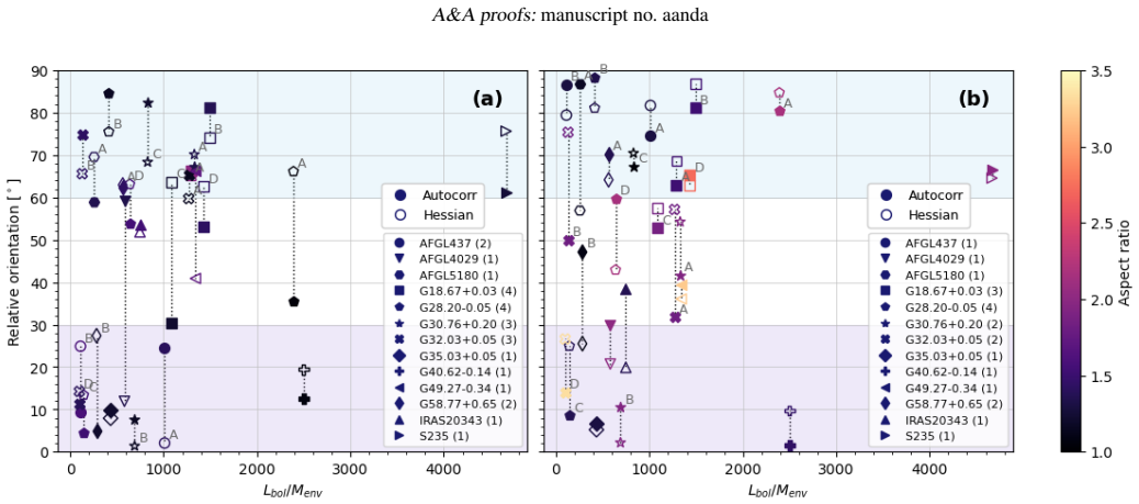
The load-bearing quantity is the relative orientation angle $\theta_{\rm rel}$, measured between the mean magnetic field orientation inside a source's optimal aperture and the structural elongation direction defined by that same aperture. The mean field direction comes from a weighted circular mean of polarization angles rotated by 90 degrees (elongated dust grains emit with their long axes perpendicular to the field); the elongation comes from two independent techniques, Hessian matrix analysis of the Stokes I map and the autocorrelation function of Stokes I with ellipse fitting, so any claimed bimodality must survive a change of method. Parallel alignment is defined as $\theta_{\rm rel}$ within $0^\circ$–$30^\circ$ and perpendicular as $60^\circ$–$90^\circ$. Statistical significance is judged against a uniform distribution on $[0^\circ, 90^\circ]$ using a one-sample Kuiper test, backed by Monte Carlo trials ($10^6$ draws) that count how often a random histogram produces as large a fraction of near-parallel and near-perpendicular sources as the data show.
What would settle it
Re-run the one-sample Kuiper and Monte Carlo tests on the source-scale relative orientation with orientation uncertainties propagated (for example, from the scatter of the autocorrelation ellipse fits across contour levels, or by restricting to sources with aspect ratio above 1.3): if the bimodality no longer reaches $p \lesssim 0.05$ under either weighting, the claim that magnetic fields dynamically regulate massive cores on roughly 0.6 pc scales would lose its statistical support. A complementary check is higher-resolution sub-arcsecond polarimetry of the same cores to see whether the parallel and perpendicular classifications of the magnetic field geometry survive at smaller scales.
Extended reading notes
Core claim
The paper's central claim is a statistically significant bimodal distribution between the SOMA source orientations and the local magnetic field orientations. Inside each source's optimal aperture (typically $\lesssim 0.6$ pc), the mean magnetic field direction, inferred from 850-micron dust polarization under the standard assumption that grains align with their long axes perpendicular to the field, is either within 30 degrees of the source's long axis or within 30 degrees of perpendicular, with few sources at intermediate angles. The pattern holds across two independent structure-orientation methods (Hessian matrix analysis and autocorrelation of the Stokes I map) and two statistical tests (a one-sample Kuiper test and $10^6$-iteration Monte Carlo simulations), giving $p = 0.010/0.012$ for Hessian-derived orientations and $p = 0.050/0.045$ for autocorrelation-derived orientations. The same analysis at the larger filament scale shows no significant bimodality ($p \gtrsim 0.1$), which the authors attribute to noisier, more diffuse emission defining the filaments. In the authors' framing, the bimodality means magnetic fields play a dynamically important, regulative role in high-mass star-forming regions, similar to results previously reported for low-mass regions.
Load-bearing premise
The results depend on treating each source's measured elongation direction as accurate, yet several sources are nearly round (aspect ratio as low as 1.04) and have essentially undefined long axes; if the uncertainty or systematic bias in these structural orientations is comparable to the 30-degree bins used to define parallel and perpendicular, the bimodality could be an artifact of the measurement rather than a real property of massive cores.
Editorial extensions
If this is right
- Magnetic fields are dynamically important on the roughly 0.6 pc scales of massive protostellar cores, favoring core-accretion models in which fields regulate collapse and fragmentation over models that ignore them.
- The bimodal alignment pattern previously found in low-mass Gould Belt clouds now extends to the high-mass regime, implying a common magnetic-regulation mechanism across stellar masses.
- Grain alignment persists up to the highest intensities probed (the $p'$–$I$ index $\alpha \approx 0.6$–$0.8$ at high intensity), so polarized dust emission remains a usable magnetic field tracer in dense massive cores.
- The significant anti-correlation between debiased polarization fraction and $L_{\rm bol}/M_{\rm env}$ means observable polarization properties systematically change as a protostar evolves.
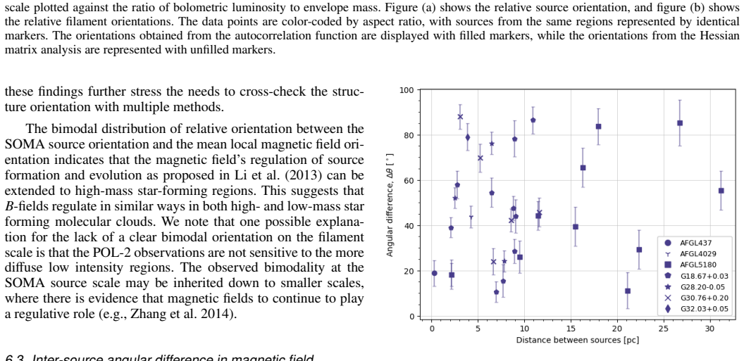
- The lack of bimodality at filament scales and of inter-source field correlations suggests that on larger scales, gravity-driven motions in the protocluster potential take over from magnetic regulation.
Reading between the lines
- Editorial extension: the bimodality predicts a resolvable morphological dichotomy at sub-arcsecond scales—parallel-class cores should show fields running along the long axis (gas accumulating along field lines) and perpendicular-class cores should show fields draped across the core (field-guided compression)—which higher-resolution interferometric polarimetry could test directly.
- Editorial extension: the cleanest internal check is to restrict the Kuiper and Monte Carlo statistics to sources with well-defined long axes (aspect ratio > 1.3); the sample's nearly round sources, such as G28.20 A at 1.04, make the current significance partly dependent on measuring a direction that is almost undefined.
- Editorial extension: the opposite-signed $p'$–dispersion trend relative to low-mass regions is plausibly driven by noisier, lower-intensity sightlines in this sample; re-binning the data at matched signal-to-noise would reveal whether the trend is a Ricean noise effect or a physical difference.
- Editorial extension: if the $p'$–$L_{\rm bol}/M_{\rm env}$ anti-correlation strengthens with a larger sample, polarization fraction could serve as a cheap evolutionary-stage diagnostic for massive protostars, complementing SED-based classification.
Editorial analysis
A structured set of objections, weighed in public.
Referee Report
Summary. The paper presents JCMT POL-2 850 µm polarization observations of 13 SOMA massive star-forming regions, yielding 29 massive protostars. It derives mean magnetic field orientations, polarization fractions, angular dispersions, and structural orientation angles via Hessian matrix and autocorrelation analyses, and compares these with SED-derived protostellar properties. The main claimed result is a statistically significant bimodal distribution of the relative orientation between the local magnetic field and the source elongation on SOMA-aperture scales (Kuiper/Monte Carlo p ≈ 0.01–0.05), while no bimodality is found for filament-scale alignment. Secondary results include a p′–I power-law slope α ≈ 0.6–0.8 at high intensity, correlations between polarization fraction/dispersion and intensity, and a reported anti-correlation between p′ and Lbol/Menv.
Significance. If the bimodality is robust, this would be an important extension of the low-mass Gould Belt cloud-field alignment results to high-mass protostellar cores, supporting a dynamically important role for magnetic fields in massive star formation. The paper's strengths are the direct POL-2 survey of a well-studied SOMA sample, the use of two structural orientation estimators, and the quantitative comparison against uniform distributions with both Kuiper and Monte Carlo tests. The SED modeling connects polarization properties to evolutionary stage. The main caveats are that the formal test treats orientation angles as exact and the autocorrelation p-value sits at the conventional threshold; these need to be addressed before the central claim is fully load-bearing.
major comments (3)
- [§6.2.1, Tables 4–5] The p-values in Table 5 are computed treating each source elongation angle as exact, but Table 4 provides no per-source uncertainty for the Hessian orientations and the autocorrelation orientations vary by tens of degrees across contour levels; several sources have aspect ratios close to unity (G28.20 A: 1.04; G40.62: 1.07; G32.03 A: 1.14). Because the parallel/perpendicular classification uses 30° bins, an orientation error of roughly 30° can move a source between bins; for example, AFGL 5180 A has θrel,SOMA ≈ 69.5° from the Hessian method and ≈59.1° from the autocorrelation method, straddling the 60° boundary. The paper should propagate orientation uncertainties into the statistical test (e.g., Monte Carlo resampling of orientations using the contour-level scatter and cross-method differences, or repeating the test after excluding low-aspect-ratio sources) and should report region-level bootstrap p-values. Until this is done, the p=0.050/0.045 autocorrelation result does not robustly support the word “statistically confirm” in the abstract.
- [§6.5, Table 6, Abstract] The Spearman test for p′ versus Lbol/Menv gives p=0.052, which is not below the conventional 0.05 threshold; the abstract's claim of a “statistically significant anti-correlation” is therefore overstated. Please either adopt an explicitly justified one-sided test, report an effect size with its uncertainty, or soften the wording so that it accurately reflects the marginal significance.
- [§6.2.1] The claim that the bimodality is confirmed “independent of the methods to measure structural orientation” is stronger than the evidence supports, because the Hessian and autocorrelation methods use the same Stokes I maps, the same apertures, and the same noise realization; agreement between them cannot remove a systematic bias shared by both. In addition, the 29 sources come from only 13 regions and are not fully independent, so the effective sample size is smaller than 29. A region-level bootstrap or a mixed-effects treatment should be added before claiming method independence.
minor comments (4)
- [Fig. 5 caption, §6.2.1] The text refers to panels “3c)” and “3d)” when describing Figure 5; these should be panels (c) and (d) of Figure 5.
- [§6.2] The sentence “Only data points with SNRI < 10 are used here as well” appears to be a typo; given the earlier masking it should presumably read SNR I > 10.
- [Table 3, G28.20 B] The equally weighted mean field orientation for G28.20 B is listed as −84.7° while the intensity-weighted value is 34.9°; this large difference should be verified and the table should clarify how angle wraparound is handled.
- [Table 7, §6.6] The source is named “G28.8 A” in Table 7 and in the text of §6.6, but everywhere else in the paper it is G28.20 A; please make the naming consistent.
Circularity Check
No circularity: the bimodality test compares independently measured polarization and column-density orientations against a uniform null; no fitted parameter is relabeled as a prediction.
full rationale
The paper's central claims are derived from independent observables and null-hypothesis tests. Magnetic field orientations come from POL-2 Stokes Q/U maps (Eqs. 1-3), source and filament elongations come from Hessian matrix and autocorrelation analyses of Stokes I maps, and the statistical significance of the resulting bimodal distribution is assessed with a one-sample Kuiper test against an analytic uniform CDF and with Monte Carlo simulations that draw random orientations from a uniform distribution. No equation in the paper reduces a predicted quantity to an input by construction: the SED-derived Lbol, Menv, and Lbol/Menv values come from a separate radiative transfer grid (Zhang & Tan 2018) implemented via sedcreator, not from the polarization data, and the p'-I power-law slopes and dispersion correlations are descriptive fits rather than fitted parameters presented as independent predictions. Self-citations appear (e.g., SOMA survey, Zhang & Tan 2018 grid, earlier work by Law et al.), but they supply context, data, or modeling tools; the load-bearing bimodality result is tested against a uniform null and does not depend on those citations as proof. The concern that near-circular sources (aspect ratios close to 1) have poorly constrained orientation angles is a measurement-uncertainty or robustness issue, not a circularity of the derivation chain.
Assumptions & free parameters
free parameters (3)
- Break point of p'-I broken power law =
not stated numerically, identified by eye in Fig. 4
- Bimodality bin boundaries =
0-30 deg (parallel), 60-90 deg (perpendicular)
- Gaussian fit parameters for theta_rel histograms =
means and dispersions in Fig. 5 legends
assumptions (4)
- domain assumption Dust grains have their long axes aligned perpendicular to the magnetic field (RAT alignment), so theta_B = theta_p + 90 degrees (Eq. 3).
- domain assumption The SOMA aperture, defined by 70 micron flux convergence, encloses the core whose orientation is compared to the B-field.
- domain assumption The Zhang & Tan (2018) turbulent core accretion model grid provides reliable Lbol and Menv estimates.
- standard math Uniform distribution is the appropriate null hypothesis for the relative orientation test.
Cite this review
Pith. "Pith review of The SOMA-POL Survey. I. Polarization and magnetic field properties of massive protostars." pith.science (2026). https://pith.science/paper/MY54YRGD
@misc{pith2026250702384,
  author       = {Pith},
  title        = {Pith review of: The SOMA-POL Survey. I. Polarization and magnetic field properties of massive protostars},
  year         = {2026},
  howpublished = {\url{https://pith.science/paper/MY54YRGD}},
  note         = {Machine review of arXiv:2507.02384}
}
abstract
The role of magnetic fields in regulating the formation of massive stars remains much debated. Here we present sub-millimeter polarimetric observations with JCMT-POL2 at $850\:\mu$m of 13 regions of massive star formation selected from the SOFIA Massive (SOMA) star formation survey, yielding a total of 29 massive protostars. Our investigation of the $p'-I$ relationship suggests that grain alignment persists up to the highest intensities. We examine the relative orientations between polarization-inferred magnetic field direction and source column density elongation direction on small and large scales. On small scales, we find a bimodal distribution of these relative orientations, i.e., with an excess of near-parallel and near-perpendicular orientations. By applying a one-sample Kuiper test and Monte Carlo simulations to compare to a relative orientation distribution drawn from a uniform distribution, we statistically confirm this bimodal distribution, independent of the methods to measure structural orientation. This bimodal distribution suggests that magnetic fields are dynamically important on the local scales ($\lesssim 0.6\:$pc) of massive protostellar cores. We also examine how basic polarization properties of overall degree of polarization and local dispersion in polarization vector orientations depend on intrinsic protostellar properties inferred from spectral energy distribution (SED) modeling. We find a statistically significant anti-correlation between the debiased polarized fraction and the luminosity to mass ratio, $L_{\rm bol}/M_{\rm env}$, which hints at a change in the dust properties for protostellar objects at different evolutionary stages.
Figures


Figures from the paper (10 more)




Reference graph
Works this paper leans on
-
[1]
A., Aghanim, N., Alina, D., et al
Ade, P. A., Aghanim, N., Alina, D., et al. 2015, Astronomy & Astrophysics, 576, A105
work page 2015
-
[2]
2016, Astronomy & Astrophysics, 595, A57
Alina, D., Montier, L., Ristorcelli, I., et al. 2016, Astronomy & Astrophysics, 595, A57
work page 2016
-
[3]
2025, arXiv e-prints, arXiv:2501.13931
Alves, J., Lombardi, M., & Lada, C. 2025, arXiv e-prints, arXiv:2501.13931
arXiv 2025
-
[4]
Andersson, B., Lazarian, A., & Vaillancourt, J. E. 2015, Annual Review of As- tronomy and Astrophysics, 53, 501
work page 2015
-
[5]
A., Bate, M
Bonnell, I. A., Bate, M. R., Clarke, C. J., & Pringle, J. E. 2001, MNRAS, 323, 785
2001
-
[6]
Ching, T. C., Li, D., Heiles, C., et al. 2022, Nature, 601, 49
work page 2022
-
[7]
2024, Astronomy & Astrophysics, 682, A2 Davis Jr, L
Crowe, S., Fedriani, R., Tan, J., et al. 2024, Astronomy & Astrophysics, 682, A2 Davis Jr, L. & Greenstein, J. L. 1951, Astrophysical Journal, vol. 114, p. 206, 114, 206
work page 2024
- [8]
Show all 37 references
-
[9]
C., Telkamp, Z., et al
Fedriani, R., Tan, J. C., Telkamp, Z., et al. 2023, ApJ, 942, 7
2023
-
[10]
M., Beltrán, M
Girart, J. M., Beltrán, M. T., Zhang, Q., Rao, R., & Estalella, R. 2009, Science, 324, 1408
2009
-
[11]
2018, arXiv preprint arXiv:1811.03100 Grudi´c, M
Gordon, M., Lopez-Rodriguez, E., Andersson, B.-G., et al. 2018, arXiv preprint arXiv:1811.03100 Grudi´c, M. Y ., Guszejnov, D., Offner, S. S. R., et al. 2022, MNRAS, 512, 216
2018 arXiv
-
[12]
Gu, Q. et al. 2019, The Astrophysical Journal Letters, 871, L15
2019
-
[13]
Kunz, M. W. & Mouschovias, T. C. 2009, MNRAS, 399, L94
2009
-
[14]
2020, Monthly Notices of the Royal Astronomical Society, 498, 850
Law, C.-Y ., Li, H.-B., Cao, Z., & Ng, C.-Y . 2020, Monthly Notices of the Royal Astronomical Society, 498, 850
2020
-
[15]
Y ., Li, H
Law, C. Y ., Li, H. B., & Leung, P. 2019, Monthly Notices of the Royal Astro- nomical Society, 484, 3604
2019
-
[16]
C., Gorai, P., et al
Law, C.-Y ., Tan, J. C., Gorai, P., et al. 2022, The Astrophysical Journal, 939, 120
2022
-
[17]
C., Skalidis, R., et al
Law, C.-Y ., Tan, J. C., Skalidis, R., et al. 2024, The Astrophysical Journal, 967, 157 Le Gouellec, V . J., Maury, A., Guillet, V ., et al. 2020, Astronomy & Astrophysics, 644, A11
2024
-
[18]
2014, Protostars and planets VI, 101
Li, H., Goodman, A., Sridharan, T., et al. 2014, Protostars and planets VI, 101
2014
-
[19]
2013, Monthly Notices of the Royal Astronomical Society, 436, 3707
Li, H.-b., Fang, M., Henning, T., & Kainulainen, J. 2013, Monthly Notices of the Royal Astronomical Society, 436, 3707
2013
-
[20]
2017, Nature Astronomy, 1, 0158
Li, H.-b., Jiang, H., Fan, X., Gu, Q., & Zhang, Y . 2017, Nature Astronomy, 1, 0158
2017
-
[21]
C., De Buizer, J
Liu, M., Tan, J. C., De Buizer, J. M., et al. 2020, The Astrophysical Journal, 904, 75
2020
-
[22]
McKee, C. F. & Tan, J. C. 2002, Nature, 416, 59
2002
-
[23]
McKee, C. F. & Tan, J. C. 2003, The Astrophysical Journal, 585, 850
2003
-
[24]
2021, The Astrophysical Journal, 922, 210
Panopoulou, G., Dickinson, C., Readhead, A., Pearson, T., & Peel, M. 2021, The Astrophysical Journal, 922, 210
2021
-
[25]
2022, arXiv preprint arXiv:2203.11179
Pattle, K., Fissel, L., Tahani, M., Liu, T., & Ntormousi, E. 2022, arXiv preprint arXiv:2203.11179
2022 arXiv
-
[26]
2019, The Astrophysical Journal, 880, 27
Pattle, K., Lai, S.-P., Hasegawa, T., et al. 2019, The Astrophysical Journal, 880, 27
2019
-
[27]
C., et al
Pillai, T., Kauffmann, J., Tan, J. C., et al. 2015, ApJ, 799, 74 Planck Collaboration, Ade, P. A. R., Aghanim, N., et al. 2015, A&A, 576, A104
2015
-
[28]
& Walch, S
Seifried, D. & Walch, S. 2015, Monthly Notices of the Royal Astronomical So- ciety, 452, 2410
2015
-
[29]
1962, in Advances in Astronomy and Astrophysics, V ol
Serkowski, K. 1962, in Advances in Astronomy and Astrophysics, V ol. 1 (Else- vier), 289–352
1962
-
[30]
D., Beuther, H., Rugel, M., et al
Soler, J. D., Beuther, H., Rugel, M., et al. 2019, A&A, 622, A166
2019
-
[31]
D., Beuther, H., Syed, J., et al
Soler, J. D., Beuther, H., Syed, J., et al. 2020, Astronomy & Astrophysics, 642, A163
2020
-
[32]
D., Hennebelle, P., Martin, P
Soler, J. D., Hennebelle, P., Martin, P. G., et al. 2013, ApJ, 774, 128
2013
-
[33]
C., Beltrán, M
Tan, J. C., Beltrán, M. T., Caselli, P., et al. 2014, Protostars and Planets VI, 149
2014
-
[34]
C., et al
Telkamp, Z., Fedriani, R., Tan, J. C., et al. 2025, The Astrophysical Journal, 986, 15
2025
-
[35]
C., Christie, D., et al
Wu, B., Tan, J. C., Christie, D., et al. 2017, ApJ, 841, 88
2017
-
[36]
M., et al
Zhang, Q., Qiu, K., Girart, J. M., et al. 2014, ApJ, 792, 116
2014
-
[37]
& Tan, J
Zhang, Y . & Tan, J. C. 2018, The Astrophysical Journal, 853, 18 Article number, page 14 of 17 T. Källberg et al.: SOMA-POL I Fig. 12. The figure illustrates the θOutflow for the four sources. The blue dashed line shows the blue-shifted outflow orientation. The pink dashed lin...
2018
Reviewed August 6, 2026 · model on record in the stance chip above.
Discussion (0). Continue with ORCID to comment.