REVIEW 3 major objections 4 minor 19 references
Vortex topology in the lee of a 6:1 prolate spheroid
T0 review · 3 major / 4 minor · reviewed 2026-08-06 · deepseek-v4-flash
Pith's one-line read Across 48 large-eddy simulations of a 6:1 prolate spheroid, the lee-side boundary layer always separates symmetrically, and the recirculation is always one of three states: a proto-vortex, a coherent vortex, or a recirculating wake.
desk verdict A genuinely useful 48-case LES taxonomy of leeward flow on the 6:1 spheroid, undermined by an algebraic error in the threshold that defines its headline scalings. read the letter →
The pith
A machine-rendered reading of the paper's core claim, the machinery that carries it, and where it could break.
The reading
What carries the argument
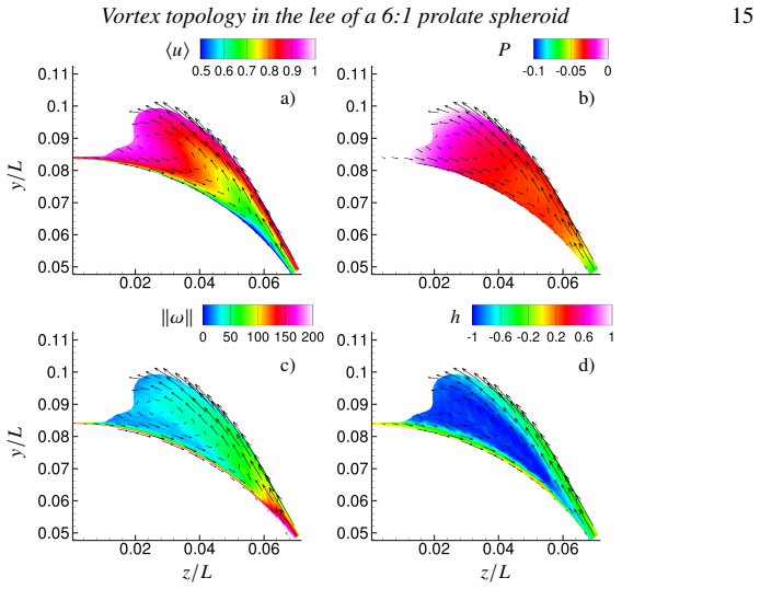
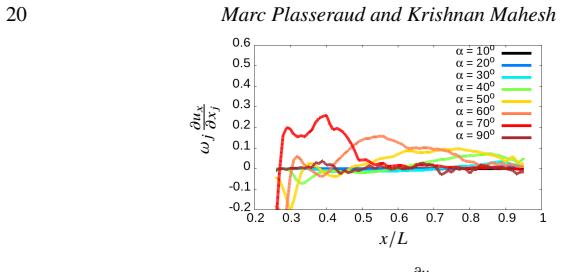
The central object is the coherent vortex, identified by the largest closed iso-surface of stagnation pressure; this definition supplies a stable boundary for measuring radius, circulation, and area. The argument's engine is an axial control-volume balance in which the constant-stagnation-pressure vortex boundary acts as a material surface, so the mass added across the separated shear layer per unit length drives the axial mass flow to grow linearly while the separation-length geometry ($L_s \sim x$) makes the area grow quadratically. The load connection comes from a Riabouchinsky-style balance between shear-layer stress and wall suction, and from Crocco's equation expressing the in-plane vortex force as the Lamb-vector integral, which isolates the left/right turbulent-stress asymmetry as the only contributor.
What would settle it
A wind-tunnel test on a 6:1 prolate spheroid at Re=1.5M and 2.5M, alpha=20 and 40 degrees, measuring the azimuthal separation line and the presence or absence of a coherent lee vortex: the paper predicts a sharp boundary-layer-state jump between those Reynolds numbers, so if the separation-line shift or vortex state is identical at both, the central Re-dependence claim is wrong.
Extended reading notes
Core claim
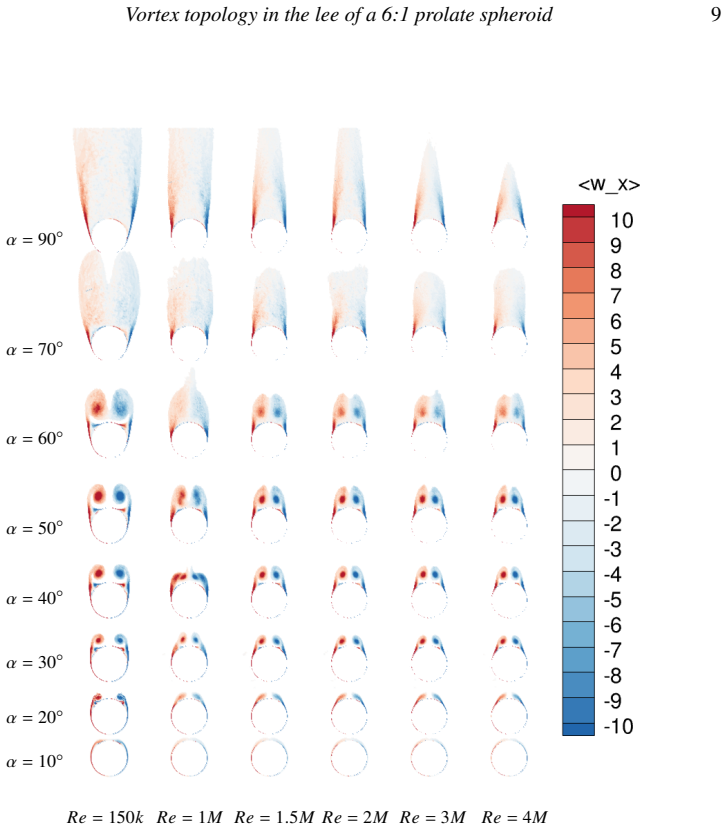
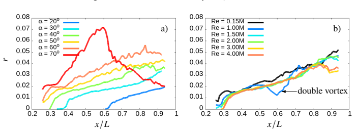
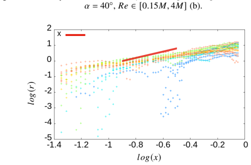
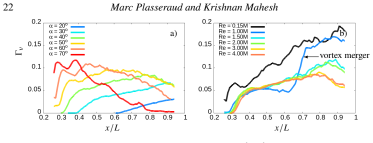
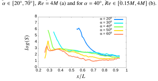
For all 48 combinations of Reynolds number and angle of attack considered, the boundary layer of the inclined 6:1 prolate spheroid separates symmetrically and its leeward recirculation belongs to one of three categories: proto-vortex, coherent vortex, or recirculating wake. In the coherent-vortex state, the separated shear layer rolls into a three-dimensional vortex aligned with the spheroid axis, whose center is a pressure minimum and which converts azimuthal momentum into axial momentum. Along the axis, the total recirculation area grows as $A_t \sim x^2$ while the total circulation grows roughly as $\Gamma_t \sim x$, with the exponent depending on angle of attack. The paper further shows that the normal force and pitching moment follow from this axial evolution: suction is highest where swirl and vortex stretching are greatest, not where the recirculation is largest, and the overturning moment comes from the first half of the body.
Load-bearing premise
The boundary-layer state at separation is the paper's explanatory variable for topology and Re-dependence, but that state is produced by dynamic-Smagorinsky LES with a trip inherited from prior work, not by resolving or modeling laminar-to-turbulent transition; if the LES misplaces transition, the separation lines, state boundaries, and Re-dependence of loads are all affected.
Editorial extensions
If this is right
- At fixed Reynolds number and incidence, the lee-side suction and lift are larger on the forward half of the spheroid, which produces the overturning pitching moment despite the body's nose-tail symmetry.
- Increasing angle of attack raises normal force up to about 70 degrees; beyond that the vortex loses coherence and suction drops.
- Increasing Reynolds number delays separation and shrinks the recirculation, lowering lift at a given incidence.
- The quadratic area growth with near-linear circulation growth implies a decreasing mean axial velocity and swirl along the vortex, consistent with the observed decay of vortex strength toward the tail.
- The three-state classification (proto-vortex, coherent vortex, recirculating wake) is exhaustive for the studied range, so a simulation or experiment at any new point in this Re-alpha range should land in one of these states.
Reading between the lines
- Editorial inference: the same three-state classification and area/circulation scaling may apply to other slender axisymmetric bodies at incidence; a quick test would be to compute $A_t(x)$ and $\Gamma_t(x)$ for a 3:1 ellipsoid or a submarine-like hull.
- Editorial inference: the finding that suction tracks swirl rather than recirculation size suggests a control-surface design rule: to maximize side force, promote early vortex inception and high swirl, not a large recirculation bubble.
- Editorial inference: because the paper's boundary-layer state is produced by an inherited trip, a transition-resolving simulation at Re=1.5M-2.5M would either confirm or shift the state boundaries and the inferred critical Reynolds number.
Editorial analysis
A structured set of objections, weighed in public.
Referee Report
Summary. The paper presents a parametric large-eddy simulation study of flow over a 6:1 prolate spheroid at six Reynolds numbers (Re = 0.15M, 1M, 1.5M, 2M, 3M, 4M) and eight angles of attack (alpha = 10 to 90 deg). The authors classify the leeward recirculation into three states (proto-vortex, coherent vortex, recirculating wake) and describe how the axial evolution of vortex radius, circulation, stagnation pressure, and swirl changes with Reynolds number and incidence. They connect these flow-topology features to the normal force and pitching moment using a control-volume mass balance and a Riabouchinsky-type cavity model, and report power-law scalings A_t ~ x^2 for recirculation area and Gamma_t ~ x^alpha for total circulation. The central claims are that separation is always symmetric in the investigated parameter range, that the coherent-vortex state converts azimuthal momentum into axial momentum, and that maximum suction occurs where swirl is high rather than where recirculation is largest.
Significance. If the quantitative results hold, the paper provides a valuable taxonomy and a large, openly described LES dataset for a canonical separated flow, building on a novel stagnation-pressure-based vortex definition (Plasseraud & Mahesh 2024a). The grid-convergence check (Table 1, 218M vs 470M: 0.11% difference in normal force) and the use of multiple consistent observables (vorticity, stagnation pressure, skin friction, helicity) lend qualitative support to the three-state classification. However, the quantitative layer--quadratic area growth, circulation scaling, and the load-topology link--is built on a threshold derived in Section 3.6 that appears to contain an algebraic error, and the Reynolds-number dependence rests on an assumed transition location that the LES does not resolve. These concerns are central to the paper's main claims, not peripheral. The qualitative taxonomy and the dataset itself are likely to be useful to the community even if the specific scalings require revision.
major comments (3)
- [Section 3.6] The derivation of the recirculation threshold P_s ≈ 0.49 P_inf_s is algebraically inconsistent. From P_s = P + 1/2 ρ u^2 and u^2/u_p^2 = 0.992, the exact expression is P_s = 0.008 P + 0.992 P_inf_s. The stated approximation P_s ≈ 0.49 P_inf_s would require P ≈ −63 P_inf_s, which is unphysical. Moreover, the factor 0.992 does not follow from the 0.01 tolerance in Section 3.5; the consistent value would be u^2/u_p^2 = (0.99)^2 = 0.9801. This threshold is load-bearing: it defines A_t (used for the x^2 scaling in Section 5.7 and Figures 39–40), the total circulation Γ_t (Figures 41–42), the primary-vortex boundary in Section 3.7, and the load integral f_y^recirculation(x) = ∫(0.49 P_inf_s − p_wall) dφ in Section 5.9.2. The authors should either correct the derivation or demonstrate that the reported scalings and load conclusions are insensitive to the threshold choice, for example by recomputing A_t, Γ_t, and the load integral for thresholds of 0.4 and 0.6 P_inf_s.
- [Section 5.2.2] The attribution of the jump in δ99 and Re_θ between Re = 1M and 1.5M to a laminar-to-turbulent transition at Re ≈ 1.5M conflicts with the cited experimental critical regime of Re = 2–3M (Ahn 1992) and with the authors' own earlier finding that trips do not guarantee a turbulent boundary layer at high incidence (Plasseraud et al. 2023). The LES uses a dynamic-Smagorinsky SGS model with a trip inherited from prior work, so the transition location is not resolved or independently modeled. The separation lines (Figures 6 and 9), the boundary-layer state (Figures 10–11), and the load trends (Figures 48–49) all depend on this assumed transition. Please provide a sensitivity check, such as a comparison against experimental separation locations in the critical regime, or discuss how the main conclusions would change if transition occurs at Re = 2–3M rather than at 1.5M.
- [Section 5.7] The control-volume mass balance that leads to the quadratic growth of A_t assumes that the surface S_Ps, an iso-surface of constant stagnation pressure, is a material surface with zero mass flux. In the turbulent, time-averaged flow considered here, the mean stagnation pressure is not constant along mean streamlines because of Reynolds stresses, and the mean mass flux across the iso-surface need not vanish. The authors state that this holds in the inviscid limit, but the LES flow is viscous and turbulent. Please quantify the neglected turbulent flux across S_Ps using the LES data (for example, by computing the actual mean normal velocity on the iso-surface), or provide a justification that the error is small enough to support the derived scaling.
minor comments (4)
- [Introduction / Section 5.4] The Introduction states that 'the primary vortex is attached and coherent at low angles of attack (10°, 20°)', but Section 5.4 classifies the 20° case as a proto-vortex without a distinct center of rotation; please reconcile this terminology.
- [Section 5.5.2] The Burgers vortex profile is written as (u_x, u_theta, u_r) = (−a r, ..., 2 a z); the radial and axial components appear to be interchanged, since a standard Burgers vortex has u_r = −a r and u_z = 2 a z.
- [Section 3.6] The notation for the freestream stagnation pressure appears both as P∞s and P_inf_s in different places; please unify the notation.
- [Figure 10] The y-axis label of Figure 10 is ambiguous; please state the units and whether the value is normalized by L.
Circularity Check
The 0.49 P∞_s recirculation threshold is asserted to follow from the δ99 definition but is algebraically unjustified; this threshold then reappears as the 'constant stagnation pressure' shear layer and enters the load/topology force integral, making part of the load–topology link definitional rather than a derived result.
-
self definitional
[Section 3.6 and Section 5.9.2]
"the separated region is defined as the area where 𝑃𝑠 < 0.49𝑃∞𝑠 and 𝑟 >𝛿99. ... In the proto–vortex and 3D vortex states, the stagnation pressure is constant at 𝑃𝑠 = 0.49𝑃∞𝑠 along the separated shear layer but has higher values in the vicinity of the meridian plane."
The later statement that stagnation pressure is constant along the separated shear layer restates the threshold used to define the recirculation boundary: the outer edge of the region 𝑃𝑠 < 0.49𝑃∞𝑠 is necessarily the 0.49 isosurface. This definitional constancy is then used in the Riabouchinsky-style load balance, with f_y^recirculation(x) = ∫(0.49𝑃∞𝑠 − 𝑝_wall)d𝜙. Thus the claim that suction from the recirculation scales with its width, and the explanation of where suction peaks, are partly built into the chosen boundary definition rather than being an independent physical finding. The wall pressure distribution itself is independent LES data, so the circularity is partial.
-
other
[Section 3.6]
"since we have ®𝑢·®𝑢/𝑢2 𝑝 =®𝑢·®𝑢/(2(𝑃∞𝑠 −𝑃)) = 0.992, the following threshold on 𝑃𝑠 could be taken: 𝑃𝑠 =𝑃(1.0− 0.992)+ 0.992𝑃∞𝑠 ≈ 0.49𝑃∞𝑠"
The algebra does not support the 0.49 value: with the factor 0.992, the expression gives 0.008𝑃 + 0.992𝑃∞𝑠, and equating this to 0.49𝑃∞𝑠 would require 𝑃 ≈ −63𝑃∞𝑠, an unphysical condition not stated or derived. The 0.49 threshold is therefore an arbitrary input presented as consistent with the δ99 boundary-layer definition. Since the same threshold defines the recirculation area A_t, the closed stagnation-pressure vortex boundary, and the load integral in Section 5.9.2, the reported scalings (A_t ~ x^2, Γ_t ~ x) and the load–topology interpretation characterize a chosen iso-surface, not an independently constrained physical boundary.
full rationale
The paper's central parametric results — symmetric separation, the three topologies, separation-line trends, and the computed normal force and pitching moment — come directly from the time-averaged LES flow fields and grid convergence, not from the threshold definition. Those parts are not circular. The circularity is concentrated in the diagnostic framework: Section 3.6 defines the recirculation as the region below 0.49P∞_s, and Section 5.9.2 then treats the 0.49 isosurface as the physical shear-layer boundary, using it in the force decomposition. The threshold's claimed derivation is algebraically invalid, so the subsequent 'constant stagnation pressure' and the resulting Riabouchinsky load relation are partly self-definitional. The self-citations to Plasseraud & Mahesh (2024a,b) supply the vortex-boundary and material-surface method; these are method citations rather than uniqueness theorems, and the material-surface property is a standard Bernoulli/Crocco consequence. The moderate score of 4 reflects that the load–topology link is partially built into the definition, while the bulk of the empirical Reynolds-number/angle-of-attack mapping remains independent LES content.
Assumptions & free parameters
free parameters (1)
- Recirculation stagnation-pressure threshold coefficient =
0.49 P_infinitys
assumptions (7)
- domain assumption Dynamic-Smagorinsky wall-resolved LES on the 470M-cell overset grid produces the correct boundary-layer state at separation at Re up to 4M without resolving or modeling natural transition.
- domain assumption The trip inherited from Plasseraud et al. (2023) gives a repeatable boundary-layer state and negligible port/starboard asymmetry, even at alpha = 90 deg.
- domain assumption Helicity-density sign change marks the primary separation line for all 48 cases.
- domain assumption The vortex boundary is the largest closed stagnation-pressure iso-surface (Plasseraud and Mahesh 2024a).
- domain assumption Three flow-throughs of time averaging give converged mean statistics in all topologies, including the unsteady recirculating wake.
- domain assumption In the control-volume balance, the constant-stagnation-pressure surface is material, with zero mean mass flux.
- domain assumption The Riabouchinsky force balance f_y(x) = integral over S of tau_s, proportional to L_s times tau_s, applies to the spheroid lee cavity.
Cite this review
Pith. "Pith review of Vortex topology in the lee of a 6:1 prolate spheroid." pith.science (2026). https://pith.science/paper/QUMQQ3XN
@misc{pith2026250703187,
  author       = {Pith},
  title        = {Pith review of: Vortex topology in the lee of a 6:1 prolate spheroid},
  year         = {2026},
  howpublished = {\url{https://pith.science/paper/QUMQQ3XN}},
  note         = {Machine review of arXiv:2507.03187}
}
read the original abstract
A large scale parametric study of the flow over the prolate spheroid is presented to understand the effect of Reynolds number and angle of attack on the separation, the wake formation and the loads. Large-Eddy Simulation is performed for six Reynolds numbers ranging from Re = 0.15M to Re = 4M and for eight angles of attack ranging from 10 degrees to 90 degrees. For all the cases considered, the boundary layer separates symmetrically and forms a recirculation region. Several distinct flow topologies are observed that can be grouped into three categories: proto-vortex, coherent vortex and recirculating wake. In the proto-vortex state, the recirculation does not have a distinct center of rotation, instead, a two-layer detached flow structure is formed. In the coherent vortex state, the separated shear layer rolls into a three-dimensional vortex that is aligned with the axis of the spheroid. This vortex has a clear center of rotation corresponding to a minimum of pressure and transforms the azimuthal momentum from the separated shear layer into axial momentum. In the recirculating wake regime, the recirculation is incoherent and the primary separation forms a dissipative shear layer that is convected in the direction of the free-stream. This symmetric pair of shear layers bounds a low-momentum recirculating cavity on the leeward side of the spheroid. The properties of these states are not constant, but evolve along the axis of the spheroid and are dictated by the characteristics of the boundary layer at separation. The variation of the flow with Reynolds number and angle of attack is described, and its connection to the loads on the spheroid are discussed.
Figures


Figures from the paper (46 more)











Reference graph
Works this paper leans on
-
[1]
1992 An experimental study of flow over a 6 to 1 prolate spheroid at incidence
Ahn, S. 1992 An experimental study of flow over a 6 to 1 prolate spheroid at incidence. PhD thesis, Virginia Polytechnic Institute and State University. Anderson, Philip W 1966 Considerations on the flow of superfluid helium. Reviews of Modern Physics 38 (2),
work page 1992
-
[2]
Kumar, P. & Mahesh, K. 2017 Large eddy simulation of flow over an axisymmetric body of revolution. Journal of Fluid Mechanics . Leasca, Theo JT, Kroll, Thomas B & Mahesh, Krishnan 2025 Large-eddy simulation of the tip vortex flow in a ducted propulsor. Journal of Fluid Mechanics 1010, A51. Lee, Mario & Ho, Chih-Ming 1990 Lift force of delta wings. Applied...
work page 2017
-
[16]
Kim, S. E., Rhee, Shin & Cokljat, D. 2003 Application of modern turbulence models to vortical flow around a prolate spheroid. In 41st Aerospace Sciences Meeting and Exhibit, p
work page 2003
-
[29]
Williamson, Charles HK1995 Vortex dynamics in the wake of a cylinder. InFluid vortices, pp. 155–234. Springer. Wu, J-Z, Lu, X-Y & Zhuang, L-X2007 Integral force acting on a body due to local flow structures.Journal of Fluid Mechanics 576, 265–286. Xiao, Z., Zhang, Y., Huang, J., Chen, H. & Fu, S.2007 Prediction of separation flows around a 6: 1 prolate sp...
work page 2007
-
[55]
Strandenes, H˚akon, Jiang, Fengjian, Pettersen, Bjørnar & Andersson, Helge I 2019 Near-wake of an inclined 6: 1 spheroid at reynolds number
work page 2019
-
[167]
& Fureby, C.2001 Large eddy simulation of the flow around an inclined prolate spheroid
Hedin, P., Berglund, M., Alin, N. & Fureby, C.2001 Large eddy simulation of the flow around an inclined prolate spheroid. In 39th Aerospace Sciences Meeting and Exhibit, p
work page 2001
-
[298]
Barber, K. M. & Simpson, R. L. 1990 Mean velocity and turbulence measurements of flow around a 6: 1 prolate spheroid. Tech. Rep.. Virginia Polytechnic Institute and State University. Brown Jr, CE & Michael, WH0057 1954 Effect of leading-edge separation on the lift of a delta wing. Journal of the Aeronautical Sciences 21 (10), 690–694. Cebeci, Tuncer & Mei...
work page 1990
-
[300]
Josephson, BD 1965 Potential differences in the mixed state of type ii superconductors
Journal of Fluid Mechanics 378, 19–70. Josephson, BD 1965 Potential differences in the mixed state of type ii superconductors. Phys. Lett.;(Netherlands)
work page 1965
Show all 19 references
-
[396]
Bulletin of the American Physical Society
Du, Yifan & Zaki, Tamer2023 Vorticity dynamics and josephson-anderson relation for flow over spheroid. Bulletin of the American Physical Society . El Khoury, George K, Andersson, Helge I & Pettersen, Bjørnar 2010 Crossflow past a prolate spheroid at reynolds number of 10000. J...
2010
-
[429]
Kroll, T. B. & Mahesh, K. 2022 Large-eddy simulation of a ducted propeller in crashback. Flow
2022
-
[630]
P., Fu, L
Griffin, K. P., Fu, L. & Moin, P. 2021 General method for determining the boundary layer thickness in nonequilibrium flows. Physical Review Fluids 6 (2), 024608. Guo, Pengming, Kaiser, Frieder & Rival, David E 2023 Vortex-wake formation and evolution on a prolate spheroid at s...
2021
-
[633]
& Moin, P
Mahesh, K., Constantinescu, G. & Moin, P. 2004 A numerical method for large–eddy simulation in complex geometries. Journal of Computational Physics 197:1, 215–240. Moffatt, Henry Keith & Tsinober, Arkady1992 Helicity in laminar and turbulent flow. Annual review of fluid mechan...
2004
-
[926]
Journal of Fluid Mechanics 960, A3
Plasseraud, Marc, Kumar, Praveen & Mahesh, Krishnan 2023 Large-eddy simulation of tripping effects on the flow over a 6: 1 prolate spheroid at angle of attack. Journal of Fluid Mechanics 960, A3. Plasseraud, Marc & Mahesh, Krishnan2024a Definition of vortex boundary using stag...
2023
-
[1035]
Horne, W. J. & Mahesh, K.2019a A massively-parallel, unstructured overset method for mesh connectivity. Journal of Computational Physics 376, 585–596. Horne, W. J. & Mahesh, K. 2019b A massively-parallel, unstructured overset method to simulate moving bodies in turbulent flows...
1995
-
[1299]
Chesnakas, C. J. & Simpson, R. L.1994 Full three-dimensional measurements of the cross-flow separation region of a 6:1 prolate spheroid. Experiments in Fluids 17 (1), 68–74. Chesnakas, C. J. & Simpson, R. L. 1996 Measurements of the turbulence structure in the vicinity of a 3-...
1994
-
[1616]
& Cabot, W
Germano, M., Piomelli, U., Moin, P. & Cabot, W. H. 1991 A dynamic subgrid–scale eddy viscosity model. Physics of Fluids A 3:7,
1991
-
[1760]
Goody, M., Simpson, R. L. & Engel, M. 1998 Mean velocity and pressure and velocity spectral measurements within a separated flow around a prolate spheroid at incidence. In36th AIAA Aerospace Sciences Meeting and Exhibit, p
1998
-
[3532]
& Mahesh, K
Morse, N. & Mahesh, K. 2021 Large-eddy simulation and streamline coordinate analysis of flow over an axisymmetric hull. Journal of Fluid Mechanics
2021
-
[4000]
Taneda, Sadatoshi1956 Experimental investigation of the wake behind a sphere at low reynolds numbers
AIAA Journal 57 (4), 1364–1372. Taneda, Sadatoshi1956 Experimental investigation of the wake behind a sphere at low reynolds numbers. Journal of the physical society of Japan 11 (10), 1104–1108. Truesdell, Clifford 1954 The kinematics of vorticity. Indiana University Press. Ve...
1954
Reviewed August 6, 2026 · model on record in the stance chip above.
Discussion (0). Continue with ORCID to comment.