REVIEW 3 major objections 5 minor 1 cited by
A perturbed cellular automaton with two phase transitions for the ergodicity
T0 review · 3 major / 5 minor · reviewed 2026-08-06 · deepseek-v4-flash
Pith's one-line read A one-dimensional cellular automaton whose noise-perturbed version is ergodic, then not ergodic, then ergodic again as the noise rate rises.
desk verdict First two-phase-transition PCA construction with a genuinely new mechanism, but the low-noise ergodicity proof has a load-bearing gap around the synchronized-zone barrier in Proposition 5.8. read the letter →
The pith
A machine-rendered reading of the paper's core claim, the machinery that carries it, and where it could break.
The reading
What carries the argument
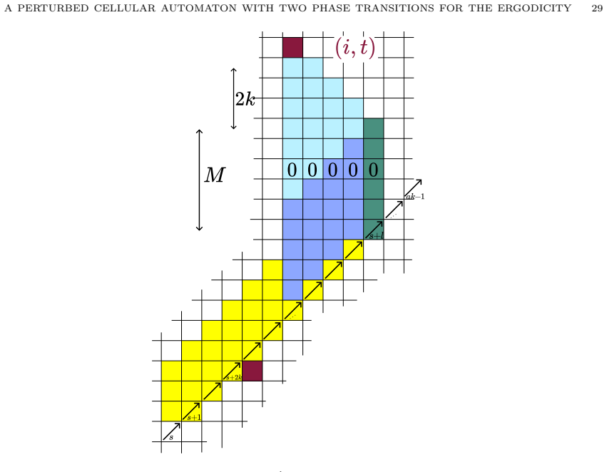
The workhorse is a two-layer update rule $T(x)_i=(G(y_{i-1},y_i,y_{i+1}),F(z)_i)$ with the caveat that when the $F$-layer produces $0$ or an arrow of type $0\bmod k$, the $G$-layer is replaced by the fixed symbol $0_G$. The $F$-layer itself is a clock: values increment mod $k$ each step, and an arrow particle $\nearrow_s$ moves right at speed 1 and resets the cells it passes to synchronized states, living at most $ak$ steps. Synchronized blocks longer than $2k$ cells reset all their $G$-layers to $0_G$ simultaneously every $k$ steps, so no radius-1 information can cross them; the paper treats this as an impenetrable wall. To turn this into a proof of ergodicity, the left and right borders of the dependence cone are bounded by Markov additive chains $(L_n,J_n)$ and $(R_n,K_n)$; the positive drift of $L_n$ and negative drift of $R_n$ follow from barrier-overcoming probabilities $\beta_\epsilon$ and success probabilities $\alpha_\epsilon$, with the barrier height $H=\ln(a)/s(\epsilon)$ chosen to make successive checks independent. Non-ergodicity at $\epsilon_2$ uses Theorem 2.1, a percolation-style condition on the error field: if every finite set $S$ has error probability at most $\epsilon_c^{|S|}$ conditional on the past, the perturbed system is non-ergodic.
What would settle it
Run the perturbation for the two chosen parameter regimes on a large finite ring: in the low-noise regime, initialize a lone synchronized block of length $2k+1$ and inject a single nonzero $G$-signal on one side immediately after a $0$-projection; if the signal appears on the other side before the next projection, the wall property is false. For the intermediate regime, check numerically whether the conditional error probability for a finite set $S$ at $\epsilon_2$ exceeds $\epsilon_c^{|S|}$ as Theorem 2.1 requires; a single counterexample to that bound would break the non-ergodicity leg.
Extended reading notes
Core claim
The central claim is Theorem 3.1: there exist integers $k,a$ and rates $0<\epsilon_1<\epsilon_2<\epsilon_3<1$ such that the uniform $\epsilon$-perturbation of a specific radius-1 cellular automaton $T$ is uniformly ergodic for all $0<\epsilon<\epsilon_1$, is not ergodic at $\epsilon_2$, and is uniformly ergodic for all $\epsilon>\epsilon_3$. The automaton is a product of two layers: an $F$-layer clock that increments modulo $k$, with right-moving arrow particles that synchronize the clocks they pass over, and a $G$-layer that is forced to a fixed symbol whenever the $F$-layer outputs $0$, so that synchronized blocks of length larger than $2k$ act as walls that stop information flow. At an intermediate rate $\epsilon_2 \sim 1/\ln\ln\ln k$, the clock layer decorrelates and the forced errors are sparse enough for the $G$-layer's built-in error correction (from the classical positive-rates counterexample, used as a black box) to preserve distant information forever, making the process non-ergodic. In the low-noise regime, arrows produced by rare errors live long and synchronize large zones, which force the dependence cone of each cell to shrink to a point almost surely; in the high-noise regime, the standard percolation argument for any perturbed cellular automaton gives ergodicity.
Load-bearing premise
The low-noise proof assumes that a contiguous block of more than $2k$ cells whose clock layer is synchronized is an impenetrable wall that no radius-1 information can cross, and this wall property is argued in a paragraph rather than isolated as a formal lemma.
Editorial extensions
If this is right
- If Theorem 3.1 is correct, the set of noise rates for which a positive-rate one-dimensional PCA is ergodic can be a non-monotone subset of $[0,1]$, not just an interval above a critical value.
- The low-noise regime is not automatically the regime where information is best preserved: here it is the regime where synchronized clock blocks scramble all transmitted information and force ergodicity.
- Because every perturbed cellular automaton is ergodic at noise rates close to 1, the new content is that non-ergodicity can occupy a middle window strictly between two ergodic regimes.
Reading between the lines
- A direct numerical test: for the $k,a$ of the construction, the survival time of arrows in the $F$-layer should grow as $\epsilon$ shrinks, and the crossing of the dependence-cone borders should occur at times consistent with the drift inequalities; measuring these in finite simulations would test the mechanism without waiting for a full proof.
- If the wall property is the weakest point, then a small modification of the $F$-layer (for example, allowing occasional errors in a synchronized block) might destroy low-noise ergodicity, which would imply the phenomenon is sensitive to the exact synchrony rather than a general principle.
- The open question posed by the authors — which subsets of $[0,1]$ can be realized as the ergodicity set of a perturbed CA — is sharpened by this example; iterating the clock-layer idea might produce three or more phase transitions, though the paper notes the construction is hard to adapt because the base automaton's invariant measures are not understood.
Signed reviews
Editorial analysis
A structured set of objections, weighed in public.
Referee Report
Summary. The paper constructs a one-dimensional probabilistic cellular automaton T_ε by coupling Gács's non-ergodic CA G with an auxiliary 'clock' layer F of counters modulo k and right-moving arrow particles. The main result (Theorem 3.1) asserts that there are parameters k,a and rates 0<ε1<ε2<ε3<1 such that T_ε is uniformly ergodic for ε∈(0,ε1), non-ergodic at ε=ε2, and uniformly ergodic for ε>ε3. The non-ergodicity regime is obtained by showing that at ε2 the errors injected into the G-layer by the F-layer plus noise satisfy the conditional probability condition of Gács's theorem (Theorem 2.1). The low-noise ergodicity regime is approached via coupling-from-the-past and dependence cones; the boundaries of the dependence cone are controlled by Markov additive chains whose positive (resp. negative) drift is computed in Sections 5.4–5.10. The high-noise regime follows from a known percolation argument. The conclusion would be the first example of two phase transitions for ergodicity in a one-dimensional PCA.
Significance. If the proof is completed, this is a substantial result: it answers a natural open question, shows that the ergodicity region in noise parameter can be disconnected, and provides a promising template for constructing multi-phase-transition PCAs by coupling a reliable automaton with a controlling layer. The paper also has clear strengths: precise definitions, a coherent overall architecture, and explicit asymptotic computations of the Markov additive chain drifts. The use of Gács's automaton as a black box is methodologically appealing. However, the significance is conditional on closing the gap concerning the synchronized-zone barrier described below.
major comments (3)
- [Section 5.3 (Proposition 5.8) and Section 5.9.2 (Proposition 5.11)] The proof of Proposition 5.8 asserts that a synchronized F-layer zone of width greater than 2k is an impenetrable barrier because 'no arrows on the F-layer cross this region.' This is not a consequence of the events G_i^t, B_i^t, O_i^t defined in Section 5.2.3: those events are formulated entirely in terms of the noise variables E_i^t being ⊥ in the green cells and the yellow triangle, and they do not constrain the F-layer configuration inherited from time -t. The F-rule gives priority to a left arrow: if z_{i-1}=↗_s then cell i becomes ↗_{s+1} regardless of its previous value. Hence an arrow initially to the left of the zone (or created by noise outside the checked region) can move into the zone without triggering any E≠⊥. When the synchronized cells next project 0_G, the cell occupied by this arrow need not project 0_G, so the wall has a moving hole and a radius-1 dependence path could cross. Since Proposition 5.8 is the only bridge from the Markov additive chain drift (inequality (5.4)) to l_t→+∞, the low-noise ergodicity leg of Theorem 3.1 does not follow. The same gap affects the right-border version (Section 5.9.2, inequality (5.8)). The authors should either prove the barrier property from the F dynamics for all configurations compatible with the noise, or enlarge the event G_i^t to exclude crossing arrows and recompute α_ε, β_ε, and the drift inequalities.
- [Section 2.2 (Theorem 2.1)] Theorem 2.1 is stated as 'a direct consequence' of the main result of [4], but no theorem or lemma number from [4] is given, and the condition 'for all finite S and all events H in the past, P(error in each cell of S | H) ≤ ε_c^{|S|}' is a strong conditional-uniform error condition. Because Section 4.4 concludes non-ergodicity of T_{ε2} from this theorem, the authors need to provide a precise reference (theorem number) and a derivation, or prove the statement. As it stands, a reader cannot verify that Gács's theorem applies to the error process produced by the F-layer plus uniform noise.
- [Section 4, opening paragraph] The sentence 'if T_{ε2} is non-ergodic on this layer, then it is non-ergodic globally' is asserted without proof. The proof that follows bounds the probability of errors in the G-coordinate, not the full-symbol errors of T_{ε2}; since Theorem 2.1 is stated for Gács's CA on alphabet G, the logical step from the G-coordinate bound to non-ergodicity of the joint system T_{ε2} on A=G×F needs to be supplied. One possible route is to argue that a G-coordinate error implies a full-symbol error and to apply a version of Gács's theorem to the joint system, but this is not written out. Please clarify this implication.
minor comments (5)
- [Section 1] The sentence 'In all known examples of CA robust to noise, there is critical value ϵc such that the perturbed cellular automaton is ergodic for any ϵ < ϵc' appears to contradict the surrounding discussion; it should presumably read 'non-ergodic for any ϵ < ϵc'.
- [Section 5.2.3] In the definitions of G_i^t and B_i^t, the condition 'n-j ≥ t-i' in the yellow triangle is not translation-invariant and is likely a typo; since these events should be invariant under spacetime translations, please replace it with the intended condition (for example n ≥ j).
- [Section 5.9.2] The sentence 'We claim that the proof of Proposition 5.8 still stands for the next proposition' should be replaced by an actual proof, especially given the issue raised in the first major comment.
- [Title and Abstract] The title and abstract contain a typo: 'PER TURBED' should be 'PERTURBED'.
- [Section 2.2] The text contains the typo 'ergordic' where 'ergodic' is intended.
Circularity Check
No significant circularity: the two phase transitions are supported by independent probabilistic estimates and an external Gács black box.
full rationale
The derivation chain of Theorem 3.1 does not reduce any of its conclusions to the assumptions by construction. The non-ergodicity leg (Section 4) verifies the conditional error-probability condition of Theorem 2.1, which is taken from Gács's external published work [4]; the parameters ϵ(k)=1/ln ln ln k and d(k)=ln ln k are chosen from independent noise estimates, and no fitted value is later renamed as a prediction. The low-noise ergodicity leg (Section 5) uses the coupling-from-the-past criterion of Proposition 5.2, cited from [10]; this is an external, published sufficient condition for uniform ergodicity and is not the target statement of this paper. The Markov additive chain drift inequalities (5.4) and (5.8) are derived from the independently defined probabilities p_good, p_bad, αϵ and βϵ, which are computed from the noise model rather than fitted to force the conclusion. The synchronized-zone barrier argument in Proposition 5.8 is asserted as a geometric consequence of the F-layer rule and the projection of 0_G; even if it is under-proved and represents a correctness or rigor concern, it is not a circular step: it does not define the target property in terms of itself, and no equation is made true by definition. The high-noise ergodicity statement is explicitly attributed to [10, Proposition 3.6] and is standard for any perturbed CA. The only self-citation is [10], which includes one author of the present paper, but its use is as a general external criterion, not as an unverified premise that is logically equivalent to the main result. Therefore no load-bearing circularity is present; the appropriate finding is a non-finding.
Assumptions & free parameters
free parameters (5)
- k
- a
- epsilon2 =
1/ln(ln(ln(k)))
- d(k) =
ln(ln(k))
- H =
ln(a)/s(epsilon)
assumptions (5)
- domain assumption Gács's theorem [4] formulated as Theorem 2.1: a PCA whose error process satisfies P(error on every cell of S | H) <= epsilon_c^{|S|} for all finite S and past events H is non-ergodic.
- domain assumption Coupling-from-the-past criterion [10, Prop 3.3]: if P(x maps to Psi^t(x; U^{-t},...,U^0)_0 is constant) tends to 1, then T_epsilon is uniformly ergodic.
- standard math Law of large numbers for Markov additive chains (Asmussen [1], ch. XI): if the mean drift kappa' > 0 then L_n tends to +infinity almost surely.
- ad hoc to paper Synchronized-zone barrier property: a synchronized block longer than 2k on the F layer blocks all radius-1 information flow on the G layer.
- domain assumption Gács CA G has radius 1 with finite alphabet; the noise model is uniform over A with an independent error field.
invented entities (1)
-
Arrow particles (rising to the right) with types 0 <= s < ak on the F layer
Cite this review
Pith. "Pith review of A perturbed cellular automaton with two phase transitions for the ergodicity." pith.science (2026). https://pith.science/paper/OGASOMMF
@misc{pith2026250703485,
  author       = {Pith},
  title        = {Pith review of: A perturbed cellular automaton with two phase transitions for the ergodicity},
  year         = {2026},
  howpublished = {\url{https://pith.science/paper/OGASOMMF}},
  note         = {Machine review of arXiv:2507.03485}
}
read the original abstract
The positive rates conjecture states that a one-dimensional probabilistic cellular automaton (PCA) with strictly positive transition rates must be ergodic. The conjecture has been refuted by G\'acs, whose counterexample is a cellular automaton that is non-ergodic under uniform random noise with sufficiently small rate. For all known counterexamples, non-ergodicity has been proved under small enough rates. Conversely, all cellular automata are ergodic with sufficiently high-rate noise. No other types of phase transitions of ergodicity are known, and the behavior of known counterexamples under intermediate noise rates is unknown. We present an example of a cellular automaton with two phase transitions. Using G\'acs's result as a black box, we construct a cellular automaton that is ergodic under small noise rates, non-ergodic for slightly higher rates, and again ergodic for rates close to 1.
Figures


Figures from the paper (11 more)




Forward citations
Cited by 1 Pith paper
-
Squeezing codes: robust fluctuation-stabilized memories
Squeezing codes are new stochastic automata that stabilize memory without symmetry, with fluctuation-stabilized order and critical exponents (z≈1.38–1.93) below the detailed-balance bound.
Reference graph
Works this paper leans on
-
[4]
Reliable Cellular Automata with Self-Organization
Peter G´ acs. “Reliable Cellular Automata with Self-Organization”. In: Journal of Statistical Physics 103 (2001), pp. 45–267
work page 2001
-
[1]
Applied Probability and Queues
Søren Asmussen. Applied Probability and Queues . Vol. 51. Stochastic Modelling and Applied Probability. New York, NY: Springer, 2003. isbn: 978-0-387-00211-8 978-0-387-21525-9. doi: 10.1007/b97236. url: http://link.springer.com/10.1007/b97236
doi:10.1007/b97236 2003
-
[2]
Reliable computation with cellular automata
P´ eter G´ acs. “Reliable computation with cellular automata”. In: J. Comput. System Sci. 32.1 (1986), pp. 15–78. issn: 0022-0000. doi: 10 . 1016 / 0022 - 0000(86 ) 90002 - 4. url: https : //doi.org/10.1016/0022-0000(86)90002-4
-
[3]
Probabilistic cellular automata with Andrei Toom
Peter G´ acs. “Probabilistic cellular automata with Andrei Toom”. English. In: Braz. J. Probab. Stat. 38.2 (2024), pp. 285–301.issn: 0103-0752. doi: 10.1214/24-BJPS605. url: projecteuclid. org/journals/brazilian- journal- of- probability- and- statistics/volume- 38/issue- 2/Probabilistic-cellular-automata-with-Andrei-Toom/10.1214/24-BJPS605.full
-
[5]
Reliable Cellular Automata with Self-Organization
Peter G´ acs. “Reliable Cellular Automata with Self-Organization”. In: arXiv e-prints (2024). arXiv: 0003117v2
work page 2024
-
[6]
Stable multi-level monotonic eroders
P´ eter G´ acs and Ilkka T¨ orm¨ a. “Stable multi-level monotonic eroders”. English. In:Theory Com- put. Syst. 66.1 (2022), pp. 322–353. issn: 1432-4350. doi: 10.1007/s00224-021-10061-w
-
[7]
A reader’s guide to P. G´ acs’s “positive rates
Lawrence F. Gray. “A reader’s guide to P. G´ acs’s “positive rates” paper: “Reliable cellular automata with self-organization” [J. Statist. Phys. 103 (2001), no. 1-2, 45–267; MR1828729 (2002c:82058a)]”. In: J. Statist. Phys. 103.1-2 (2001), pp. 1–44. issn: 0022-4715,1572-9613. doi: 10.1023/A:1004824203467. url: https://doi.org/10.1023/A:1004824203467
-
[8]
The positive rates problem for attractive nearest neighbor spin systems on Z
Lawrence F. Gray. “The positive rates problem for attractive nearest neighbor spin systems on Z”. English. In: Z. Wahrscheinlichkeitstheor. Verw. Geb. 61 (1982), pp. 389–404. issn: 0044-3719. doi: 10.1007/BF00539839
Show all 12 references
-
[9]
Thomas M. Liggett. Interacting particle systems . Classics in Mathematics. Reprint of the 1985 original. Springer-Verlag, Berlin, 2005, pp. xvi+496.isbn: 3-540-22617-6. doi: 10.1007/b138374. url: https://doi.org/10.1007/b138374
1985 doi
-
[10]
Ergodicity of some classes of cellular au- tomata subject to noise
Ir` ene Marcovici, Mathieu Sablik, and Siamak Taati. “Ergodicity of some classes of cellular au- tomata subject to noise”. In: Electronic Journal of Probability 24 (2019). Publisher: Institute of Mathematical Statistics. doi: 10.1214/19- ejp297. url: https://doi.org/10.1214%2F...
2019 doi
-
[11]
Stable and attractive trajectories in multicomponent systems
A. L. Toom. “Stable and attractive trajectories in multicomponent systems”. In: Multicomponent random systems . Vol. 6. Adv. Probab. Related Topics. Dekker, New York, 1980, pp. 549–575. isbn: 0-8247-6831-0
1980
-
[12]
Bernoulli and Markov stationary measures in discrete local interactions
N. B. Vasilyev. “Bernoulli and Markov stationary measures in discrete local interactions”. In: Developments in statistics, Vol. 1 . Academic Press, New York, 1978, pp. 99–112. Institut de Math´ematiques de Toulouse, Universit ´e Paul Sabatier, Toulouse, France Email address: h...
1978
Reviewed August 6, 2026 · model on record in the stance chip above.
Discussion (0). Continue with ORCID to comment.