REVIEW 3 major objections 7 minor 1 cited by
Bilinear Quadratic Output Systems and Balanced Truncation
T0 review · 3 major / 7 minor · reviewed 2026-08-06 · deepseek-v4-flash
Pith's one-line read Bilinear systems with quadratic outputs can be reduced by balanced truncation using newly defined algebraic Gramians and generalized Lyapunov equations.
desk verdict Solid MIMO extension of balanced truncation for bilinear quadratic output systems, with clean Gramian theory and reproducible numerics, but no error bounds and unverified smallness conditions. read the letter →
The pith
A machine-rendered reading of the paper's core claim, the machinery that carries it, and where it could break.
The reading
What carries the argument
The central object is the Volterra-series expansion of the state $x(t)=\sum_i x_i(t)$ and of the dual state, whose kernel matrices $\bar{P}_i$ and $\bar{Q}_i$ define the Gramians as infinite sums of integrals. The carrying identity is the generalized Lyapunov equation: $P$ satisfies $AP + PA^T + \sum_{k=1}^m N_k P N_k^T + BB^T = 0$, $Q_S$ satisfies $A^T Q_S + Q_S A + \sum_{k=1}^m N_k^T Q_S N_k + \sum_{j=1}^p M_j P M_j + C^T C = 0$, and $Q_A$ satisfies $A^T Q_A + Q_A A + \sum_{j=1}^p M_j P M_j + C^T C = 0$. Existence and uniqueness hinge on the operator-theoretic characterization in Theorem 4.3, applied to the linear operator $L_A(X)=AX+XA^T$ with a nonnegative perturbation $\Pi$, and on the smallness condition $\Gamma < 2\alpha/\beta^2$. Truncated Gramians replace the generalized equations by two or three standard Lyapunov equations.
What would settle it
Take a stable $A$ with known decay constants $\alpha$ and $\beta$ and choose $N_1$ and $M_1$ with norms satisfying $\Gamma \ge 2\alpha/\beta^2$; if the fixed-point iteration for $P$ or $Q_S$ still converges to a symmetric positive semidefinite solution, or if balanced truncation still matches the full output, then the stated threshold is not the true boundary of the theory.
Extended reading notes
Core claim
The paper's central claim is that a bilinear quadratic output system of the form (1.1) carries well-defined algebraic reachability and observability Gramians that are computable as limits of Volterra-series kernels and satisfy generalized Lyapunov equations. Specifically, the reachability Gramian $P$ solves $AP + PA^T + \sum_{k=1}^m N_k P N_k^T + BB^T = 0$; the standard observability Gramian $Q_S$ solves $A^T Q_S + Q_S A + \sum_{k=1}^m N_k^T Q_S N_k + \sum_{j=1}^p M_j P M_j + C^T C = 0$; and the alternative Gramian $Q_A$ solves $A^T Q_A + Q_A A + \sum_{j=1}^p M_j P M_j + C^T C = 0$. The authors prove that under the smallness condition of Theorem 4.1 these equations have unique symmetric positive semidefinite solutions, that $Q_S$ and the independently constructed $Q_P$ coincide, and that balanced truncation built from the square-root factors of $P$ and $Q$ produces a reduced BQO system whose output tracks the full output. The same Gramians recover bilinear and linear-quadratic-output systems as special cases.
Load-bearing premise
The paper assumes the bilinear and quadratic coupling matrices are small enough that the Volterra series for the state converges, quantified as $\Gamma < 2\alpha/\beta^2$; if that condition fails, the Gramians, the Lyapunov equations, and the balancing argument are undefined and no alternative is offered.
Editorial extensions
If this is right
- Reduced BQO models returned by Algorithm 6.1 keep the bilinear state equation and the quadratic output structure, so downstream tasks such as simulation, control, and optimization can treat the reduced model as a BQO system.
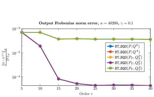
- Truncated Gramians $P_T$, $Q_T^S$, and $Q_T^P$ require only two or three standard Lyapunov solves, giving substantial speedups while matching full-Gramian accuracy in both numerical examples.
- The MIMO treatment covers systems with multiple inputs and outputs, generalizing the previous SISO analysis, with bilinear and linear-quadratic-output systems appearing as special cases.
- Because $Q_S$ satisfies a generalized Lyapunov equation while $Q_A$ solves a standard one, $Q_A$ is cheaper but provably yields smaller Hankel singular values and, in the examples, worse output fidelity.
- The mixed parameter $\phi$ in $Q_M$ interpolates between $Q_S$ and $Q_A$, and with $\phi=\gamma$ it can be interpreted as an input-scaling choice for the observability equation.
Reading between the lines
- If the smallness condition is nearly tight, rescaling inputs by $\gamma<1$ (as done in the experiments) buys existence of the Gramians but changes the input-output map; one could quantify the trade-off between the chosen $\gamma$ and the resulting reduction error.
- The $Q_A$ Gramian's failure to capture the bilinear dynamics under nonzero input suggests that $Q_A$ may still be useful for systems with weak bilinear coupling, or as a cheap initial guess for iterative solves of the $Q_S$ equation.
- The equivalence $Q_S=Q_P$ under uniqueness indicates that the two derivations are not competing, and future work could identify when the cheaper truncation $Q_T^P$ is safe, since the examples show it loses slightly at higher reduced orders.
- The same dual-system construction could be tested directly on bilinear port-Hamiltonian systems, which are a special case of (1.1), to see whether the reduced model preserves passivity or port-Hamiltonian structure.
Editorial analysis
A structured set of objections, weighed in public.
Referee Report
Summary. The manuscript treats bilinear systems with quadratic output, of the form \dot x = Ax + \sum N_k x u_k + Bu, y = Cx + [x^T M_j x]. It defines a reachability Gramian P and several observability Gramians QS, QP, QA, QM from Volterra and dual-system expansions, derives the generalized Lyapunov equations (3.6), (3.19), (3.30), (3.31), proves existence and uniqueness under explicit smallness conditions, shows QS = QP, introduces truncated Gramians that require only standard Lyapunov solves, and presents a balanced-truncation algorithm with two numerical examples. The stated goal is a structure-preserving reduced BQO model whose output tracks the full output.
Significance. The algebraic core is a useful extension of existing bilinear and LQO Gramian theories to MIMO BQO systems without the (n+n^2) lifting transformation. Strong points include explicit smallness hypotheses, a clean derivation of the Lyapunov equations from Volterra kernels, the identification QS = QP, and efficient truncated algorithms with an available implementation and reproducible code. No fitted constants enter the derivations; the user choices gamma and phi are declared as such. The numerical comparison of QS, QA, and QM is informative. The main deficiency is that the balanced-truncation step is not accompanied by any stability, error, or energy bound, and the experiments do not certify the hypotheses of Theorem 4.1, so the central reduction claim currently rests on heuristics and numerics alone.
major comments (3)
- [Section 6, Algorithm 6.1] The balanced truncation framework is presented without a stability or error theorem for the reduced BQO model (1.3). Algorithm 6.1 constructs \hat A, \hat B, \hat C, \hat N_k, \hat M_j, but nowhere is it proved that \hat A is stable, that the reduced system remains balanced in the same sense, or that \|y - \hat y\| is controlled by discarded Hankel singular values. Theorem 6.1 characterizes only the kernels of P, QS, and QA; it does not imply a reduction error bound. Since the abstract and Section 8 claim that the reduced output approximates the full output, this is a load-bearing gap. Please add such a result, even under the smallness conditions of Theorem 4.1, or explicitly label the reduction step as heuristic and supported only by experiments.
- [Section 7] The numerical experiments never report the constants needed to check the hypotheses of Theorems 4.1 and 4.4. After the gamma-scaling in Section 7, the paper states that the existence conditions are 'easier to hold', but it does not give alpha, beta, Gamma_P, Gamma_QS, or Gamma_QA for either example. If any of these inequalities fail, the algebraic solutions of (3.6), (3.19), and (3.30) may still exist, but they are not proven to coincide with the Volterra-series Gramians of Definitions 3.1, 3.3, and 3.7; consequently, the reductions depicted in Figures 1-6 and Tables 1-2 may lie outside the proven regime. Please verify the inequalities and report the values, or state explicitly that the algebraic Gramians are used by definition in the numerical part.
- [Section 5] The truncated Gramians PT, QS_T, QP_T, and QA_T are proposed as cheaper surrogates, but the paper gives no perturbation bound such as \|P - P_T\| or \|QS - QS_T\| in terms of the discarded terms P_j and QS_j. The statements in Section 5 and the Conclusion that the truncated variants 'approximate the full ones effectively' are supported only by the two examples. A bound using the smallness constants of Theorem 4.1 would make the computational shortcut rigorous; otherwise this claim should be presented as empirical.
minor comments (7)
- [Section 2 and Section 6] The symbol alpha is used both for the exponential decay rate in Theorem 4.1 and for the input-energy bound in the observability functional (6.2), which is confusing; please use two different symbols.
- [Theorem 3.4 proof] In the proof of Theorem 3.4, the notation N^T_T (presumably the transpose of the block row N^T) is never defined; please introduce a symbol such as \tilde N = [N_1; ...; N_m] once and use it consistently.
- [Section 7.1] The text states that the discrete-time output satisfies Y_i \approx y(t_i) \in \mathbb{R}^2 and Y \in \mathbb{R}^{2\times N_t}, but the RC example is SISO; these should be \mathbb{R} and \mathbb{R}^{1\times N_t}.
- [Section 7.1] The sentence 'the HSVs of the truncated variants match the HSVs of the methods using the truncated variants' appears to be a typo; presumably it should compare the truncated variants with the full-Gramian variants.
- [Figures 3 and 6] The captions of Figures 3 and 6 do not identify which line style corresponds to which method; please add a legend or describe the line styles in the captions.
- [Definition 3.7] There is an unbalanced parenthesis in the title of Definition 3.7: '(Alternative) Observability Gramian QA)' should read 'Alternative Observability Gramian QA'.
- [Algorithm 5.2] Step 2 of Algorithm 5.2 says 'Solve ... for \hat Q_S = Q_S^1 + Q_S^2'; this should be phrased as 'Solve for \hat Q_S, and set \hat Q_S = Q_S^1 + Q_S^2'.
Circularity Check
No significant circularity: the Gramians are defined from Volterra/dual expansions and their Lyapunov equations are derived by direct manipulation, with no fitted parameter relabeled as a prediction and no load-bearing self-citation.
full rationale
The paper derives the reachability Gramian P from the Volterra series solution of the BQO state equation (Definition 3.1 and Theorem 3.2), and the observability Gramians QS, QP, QM, QA from explicit dual-system Volterra constructions (Definitions 3.3, 3.5, 3.7, Theorem 3.11). The Lyapunov equations (3.6), (3.19), (3.30), and (3.31) are obtained by substituting these definitions into the integrals and using the recurrence relations for the Volterra kernels; they are not imposed as the target. The fact that QS is built using reachability kernels Pi is not circular: the dual system in (3.14) genuinely couples z to the primal trajectory x, so the observability mapping necessarily contains Pi terms, and the resulting P-dependent Lyapunov equation is a computed consequence rather than an assumption. The equality QS = QP is not assumed; it follows from Corollary 4.5 because both satisfy the same generalized Lyapunov equation whose unique symmetric positive semidefinite solution is established in Theorem 4.4 using external uniqueness theorems (Theorem 4.3). The existence conditions in Theorem 4.1 are proven by explicit norm bounds, not by citing the conclusion. The scaling parameter gamma and the mixed parameter phi in Section 7 are user-chosen and are reported as such; they are not fitted to the output data and then relabeled as predictions. The numerical experiments compare reduced outputs to full outputs, which is a standard empirical validation of the balancing construction, not a circular use of the Gramians. The only caveat worth noting is that the numerical examples do not explicitly verify that the Theorem 4.1 smallness bounds (Gamma_P, Gamma_QS, Gamma_QA < 2 alpha / beta^2) hold for the reported systems; this is a validation-gap or correctness-risk issue, not a circularity. There is no self-citation chain carrying a load-bearing argument: the cited works [10], [28], [8], [7], and [16] are independent prior results applied as standard tools. Overall, the derivation is self-contained in the sense that the claimed Lyapunov equations and existence results are derived from the definitions rather than being equivalent to the inputs by construction.
Assumptions & free parameters
free parameters (2)
- Input scaling factor gamma =
0.1 or 0.5 in the numerical examples
- Mixed Gramian weights phi_k =
0, 0.1, 0.5, 1 considered in experiments
assumptions (4)
- standard math Stability of A with decay rate constants beta and alpha such that ||e^{At}|| <= beta e^{-alpha t} for t >= 0.
- standard math Theorem 4.3 from references [7,16], characterizing existence and uniqueness for generalized Lyapunov equations via the spectrum of L_A + Pi and the spectral radius of L_A^{-1} Pi.
- domain assumption The Volterra series expansion (3.2) of the bilinear state equation converges when the smallness conditions hold.
- domain assumption The observability Gramian is defined as the reachability Gramian of the dual system, following [10,17].
Cite this review
Pith. "Pith review of Bilinear Quadratic Output Systems and Balanced Truncation." pith.science (2026). https://pith.science/paper/R2EXQWQE
@misc{pith2026250703684,
  author       = {Pith},
  title        = {Pith review of: Bilinear Quadratic Output Systems and Balanced Truncation},
  year         = {2026},
  howpublished = {\url{https://pith.science/paper/R2EXQWQE}},
  note         = {Machine review of arXiv:2507.03684}
}
read the original abstract
Dynamical systems with quadratic outputs have recently attracted significant attention. In this paper, we consider bilinear dynamical systems, a special class of weakly nonlinear systems, with a quadratic output. We develop various primal-dual formulations for these systems and define the corresponding system Gramians. Conditions for the existence and uniqueness of these Gramians are established, and the generalized Lyapunov equations they satisfy are derived. Using these Gramians and their truncated versions, which are computationally more efficient, we construct a balanced truncation framework for bilinear systems with quadratic outputs. The proposed approach is demonstrated through two numerical examples.
Figures


Figures from the paper (3 more)


Forward citations
Cited by 1 Pith paper
-
Bilinear Systems with Quadratic Outputs: $\mathcal{H}_2$ Analysis, Optimality Conditions for Model Reduction, and Algorithmic Solutions
An H2 inner product, norm, output bounds, and first-order optimality conditions are derived for bilinear systems with quadratic outputs, and an iteration (BQO-TSIA) is shown to meet the conditions upon convergence.
Reference graph
Works this paper leans on
-
[1]
L. Y. Adrianova , Introduction to linear systems of differential equations. Transl. from the Russian by Peter Zhevandrov, vol. 146 of Transl. Math. Monogr., Providence, RI: American Mathematical Society, 1995
work page 1995
-
[2]
S. Al-Baiyat and M. Bettayeb, A new model reduction scheme for k-power bilinear systems , in Proceedings of 32nd IEEE Conference on Decision and Control, Dec. 1993, pp. 22–27 vol.1, https://doi.org/10.1109/CDC.1993.325196
-
[3]
A. C. Antoulas, Approximation of Large-Scale Dynamical Systems, Society for Industrial and Applied Mathematics, 2005, https://doi.org/10.1137/1.9780898718713
-
[4]
Z. Bai and D. Skoogh, A projection method for model reduction of bilinear dynamical systems, Linear Algebra and its Applications, 415 (2006), pp. 406–425, https://doi.org/10.1016/j. laa.2005.04.032
doi:10.1016/j 2006
-
[5]
P. Benner and T. Breiten , Low rank methods for a class of generalized Lyapunov equa- tions and related issues , Numer. Math., 124 (2013), pp. 441–470, https://doi.org/10.1007/ s00211-013-0521-0. BQO SYSTEMS AND BALANCED TRUNCATION 29
work page 2013
-
[6]
P. Benner and T. Breiten , Chapter 6: Model Order Reduction Based on System Balancing , SIAM, 2017, pp. 261–295, https://doi.org/10.1137/1.9781611974829.ch6
-
[8]
P. Benner and T. Damm, Lyapunov Equations, Energy Functionals, and Model Order Reduc- tion of Bilinear and Stochastic Systems , SIAM Journal on Control and Optimization, 49 (2011), pp. 686–711, https://doi.org/10.1137/09075041X. Publisher: Society for Industrial and Applied Mathematics
-
[9]
P. Benner and H. F aßbender , Modellreduktion: Eine systemtheoretisch orientierte Einf¨ uhrung, Springer Studium Mathematik (Master), Springer Berlin Heidelberg, Berlin, Heidelberg, 2024, https://doi.org/10.1007/978-3-662-67493-2. ISSN: 2509-9310, 2509- 9329
Show all 42 references
-
[10]
Benner and P
P. Benner and P. Goyal , Balanced truncation for quadratic-bilinear control systems , Advances in Computational Mathematics, 50 (2024), p. 88, https://doi.org/10.1007/ s10444-024-10186-9
2024
-
[11]
Benner, P
P. Benner, P. Goyal, and I. P. Duff , Gramians, Energy Functionals, and Balanced Trun- cation for Linear Dynamical Systems With Quadratic Outputs , IEEE Transactions on Automatic Control, 67 (2022), pp. 886–893, https://doi.org/10.1109/TAC.2021.3086319
2022
-
[12]
Benner, P
P. Benner, P. Goyal, and M. Redmann , Truncated Gramians for Bilinear Systems and Their Advantages in Model Order Reduction , Springer International Publishing, Cham, 2017, pp. 285–300, https://doi.org/10.1007/978-3-319-58786-8 18
2017 doi
-
[13]
Breiten and T
T. Breiten and T. Stykel , Balancing-related model reduction methods, De Gruyter, Berlin, Boston, 2021, pp. 15–56, https://doi.org/doi:10.1515/9783110498967-002
2021 doi
-
[14]
Condon and R
M. Condon and R. Ivanov , Nonlinear systems – algebraic gramians and model re- duction, COMPEL - The international journal for computation and mathematics in electrical and electronic engineering, 24 (2005), pp. 202–219, https://doi.org/10.1108/ 03321640510571147
2005
-
[15]
Damm , Rational Matrix Equations in Stochastic Control , Lecture Notes in Control and Information Sciences, 297 (2004)
T. Damm , Rational Matrix Equations in Stochastic Control , Lecture Notes in Control and Information Sciences, 297 (2004)
2004
-
[16]
Damm , Direct methods and ADI-preconditioned Krylov subspace methods for generalized Lyapunov equations, Numerical Linear Algebra with Applications, 15 (2008), pp
T. Damm , Direct methods and ADI-preconditioned Krylov subspace methods for generalized Lyapunov equations, Numerical Linear Algebra with Applications, 15 (2008), pp. 853–871, https://doi.org/10.1002/nla.603
2008 doi
-
[17]
Fujimoto, J
K. Fujimoto, J. M. Scherpen, and W. Gray , Hamiltonian realizations of nonlinear adjoint operators, Automatica, 38 (2002), pp. 1769–1775, https://doi.org/https://doi.org/10.1016/ S0005-1098(02)00079-1
2002
-
[18]
G. H. Golub and C. F. V an Loan, Matrix Computations - 4th Edition , Johns Hopkins Uni- versity Press, Philadelphia, PA, 2013, https://doi.org/10.1137/1.9781421407944
2013 doi
-
[19]
W. S. Gray and J. Mesko , Energy Functions and Algebraic Gramians for Bilinear Sys- tems, IF AC Proceedings Volumes, 31 (1998), pp. 101–106, https://doi.org/10.1016/ S1474-6670(17)40318-1
1998
-
[20]
Gugercin and A
S. Gugercin and A. Antoulas, A survey of model reduction by balanced truncation and some new results, International Journal of Control, 77 (2004), pp. 748–766, https://doi.org/10. 1080/00207170410001713448
2004
-
[21]
Hartmann, C
C. Hartmann, C. Sch ¨afer-Bung, and A. Th ¨ons-Zueva, Balanced averaging of bilinear sys- tems with applications to stochastic control , SIAM J. on Control and Optimization, 51 (2013), pp. 2356–2378
2013
-
[22]
R. A. Horn and C. R. Johnson, Topics in matrix analysis. 1st paperback ed. with corrections, Cambridge: Cambridge University Press, 1st pbk with corr. ed., 1994
1994
-
[23]
Lancaster and M
P. Lancaster and M. Tismenetsky , The theory of matrices. 2nd ed., with applications , Computer Science and Applied Mathematics. Orlando etc.: Academic Press (Harcourt Brace Jovanovich, Publishers). XV (1985)., 1985
1985
-
[24]
Mehrmann and B
V. Mehrmann and B. Unger , Control of port-Hamiltonian differential-algebraic systems and applications , Acta Numerica, 32 (2023), pp. 395–515, https://doi.org/10.1017/ S0962492922000083
2023
-
[25]
Mohler , Nonlinear systems (vol
R. Mohler , Nonlinear systems (vol. 2): applications to bilinear control , Prentice-Hall, Inc. Upper Saddle River, NJ, USA, 1991
1991
-
[26]
Moore, Principal component analysis in linear systems: Controllability, observability, and model reduction, IEEE Transactions on Automatic Control, 26 (1981), pp
B. Moore, Principal component analysis in linear systems: Controllability, observability, and model reduction, IEEE Transactions on Automatic Control, 26 (1981), pp. 17–32, https: //doi.org/10.1109/TAC.1981.1102568
1981
-
[27]
Mullis and R
C. Mullis and R. Roberts , Synthesis of minimum roundoff noise fixed point digital filters , IEEE Transactions on Circuits and Systems, 23 (1976), pp. 551–562, https://doi.org/10. 30 H. F AßBENDER, S. GUGERCIN AND T. PETERS 1109/TCS.1976.1084254
1976
-
[28]
Padhi, Model Order Reduction of Nonlinear Dynamical Systems , master’s thesis, Indian Institute of Science Education and Research Pune, Pashan, Pune India, May 2024
R. Padhi, Model Order Reduction of Nonlinear Dynamical Systems , master’s thesis, Indian Institute of Science Education and Research Pune, Pashan, Pune India, May 2024
2024
-
[29]
Pulch, Energy-based model order reduction for linear stochastic Galerkin systems of second order, PAMM, 23 (2023), p
R. Pulch, Energy-based model order reduction for linear stochastic Galerkin systems of second order, PAMM, 23 (2023), p. e202300038, https://doi.org/10.1002/pamm.20230003833
2023 doi
-
[30]
Pulch and A
R. Pulch and A. Narayan , Balanced truncation for model order reduction of linear dynam- ical systems with quadratic outputs , SIAM Journal on Scientific Computing, 41 (2019), pp. A2270–A2295, https://doi.org/10.1137/17M1148797
2019 doi
-
[31]
Reiter and S
S. Reiter and S. W. R. Werner, Interpolatory model order reduction of large-scale dynamical systems with root mean squared error measures , 2024, https://arxiv.org/abs/2403.08894
2024 arXiv
-
[32]
Reiter and S
S. Reiter and S. W. R. Werner , Interpolatory model reduction of dynamical systems with root mean squared error, IF AC-PapersOnLine, 59 (2025), pp. 385–390, https://doi.org/10. 1016/j.ifacol.2025.03.066
2025
-
[33]
W. J. Rugh, Nonlinear System Theory: The Volterra/Wiener Approach , Johns Hopkins Uni- versity Press, 1981
1981
-
[34]
J. Saak, M. K ¨ohler, and P. Benner , M-M.E.S.S.-3.0 – the matrix equations sparse solvers library, Aug. 2023, https://doi.org/10.5281/zenodo.7701424. see also:https://www. mpi-magdeburg.mpg.de/projects/mess
2023 doi
-
[35]
J. M. A. Scherpen , Balancing for nonlinear systems , Systems & Control Letters, 21 (1993), pp. 143–153, https://doi.org/10.1016/0167-6911(93)90117-O
1993 doi
-
[36]
S. D. Shank, V. Simoncini, and D. B. Szyld , Efficient low-rank solution of generalized Lyapunov equations , Numer. Math., 134 (2016), pp. 327–342, https://doi.org/10.1007/ s00211-015-0777-7
2016
-
[37]
E. D. Sontag, Mathematical control theory. Deterministic finite dimensional systems. , vol. 6 of Texts Appl. Math., New York, NY: Springer, 2nd ed. ed., 1998
1998
-
[38]
V an Beeumen, K
R. V an Beeumen, K. V an Nimmen, G. Lombaert, and K. Meerbergen, Model reduction for dynamical systems with quadratic output , International Journal for Numerical Methods in Engineering, 91 (2012), pp. 229–248, https://doi.org/10.1002/nme.4255
2012 doi
-
[39]
van der Schaft, Port-Hamiltonian systems: an introductory survey , in International con- gress of mathematicians, European Mathematical Society Publishing House (EMS Ph), 2006, pp
A. van der Schaft, Port-Hamiltonian systems: an introductory survey , in International con- gress of mathematicians, European Mathematical Society Publishing House (EMS Ph), 2006, pp. 1339–1365, https://doi.org/10.4171/022-3/65
2006 doi
-
[40]
J. L. Willems , Stability Theory of Dynamical Systems , Wiley, New York, 1970
1970
-
[41]
Yue and K
Y. Yue and K. Meerbergen, Accelerating optimization of parametric linear systems by model order reduction, SIAM Journal on Optimization, 23 (2013), pp. 1344–1370, https://doi.org/ 10.1137/120869171
2013 doi
-
[42]
Zhang and J
L. Zhang and J. Lam , On H2 model reduction of bilinear systems , Automatica, 38 (2002), pp. 205–216, https://doi.org/10.1016/S0005-1098(01)00204-7
2002 doi
-
[43]
K. Zhou, J. C. Doyle, and K. Glover , Robust and optimal control, Upper Saddle River, NJ: Prentice Hall, 1996
1996
Reviewed August 6, 2026 · model on record in the stance chip above.
Discussion (0). Continue with ORCID to comment.