REVIEW 3 major objections 6 minor 1 cited by
Multi-patch/multiple-scattering frequency-time hybrid solver for interior and exterior wave equation problems
T0 review · 3 major / 6 minor · reviewed 2026-08-06 · deepseek-v4-flash
Pith's one-line read This paper proves, under a conjectured Huygens condition, that the wave trapped in a closed cavity equals a sum of multiple-scattering solutions off overlapping open arcs, for arbitrarily long times.
desk verdict Genuine N-patch generalization of the FTH solver with a clean induction proof, but the central identity rests on an unproved Huygens condition that the authors should either prove or clearly label as an assumption. read the letter →
The pith
A machine-rendered reading of the paper's core claim, the machinery that carries it, and where it could break.
The reading
What carries the argument
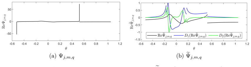
The machinery is the recursive multiple-scattering sum together with the Huygens condition that makes it agree with the true field. The boundary $\Gamma$ is covered by $N$ overlapping open arcs $\Gamma_j$ carrying a smooth partition of unity $\chi_j$; the recursion starts with $g_{j,1} = -\chi_j u^i$ and forms each later datum $g_{j,m+1} = -\chi_j \sum_{k\neq j} \tilde{v}_{k,j,m}$ from the fields arriving from the other patches, with the overlap parts set to zero so the data stay continuous and vanish at the truncated-arc endpoints. Condition 2.3, the restricted Huygens domain-of-influence condition, proven only for a flat arc and numerically demonstrated for curved arcs, asserts that data on a sub-arc away from the endpoints produce no field on the rest of the curve before time $c^{-1}\,\mathrm{dist}(C_{\text{inc}}, \text{endpoints})$; Lemma 3.1 converts this into the statement that a field from one patch cannot reach another patch before $\delta_{\min}/c$, so each scattering round extends the exactness window by exactly $\delta_{\min}/c$, and Theorem 3.5 assembles the induction (Lemma 3.4) into the identity $u = u_M$. Numerically, each open-arc round is solved by the FTH machinery of windowing-and-recentering plus high-frequency Fourier transforms, and a cosine-type change of variables (4.8) turns the endpoint and overlap-induced density singularities into smooth unknowns.
What would settle it
Place a probe on a curved open arc and illuminate only a sub-arc strictly away from both endpoints; if the scattered field at the probe turns nonzero before the elapsed time reaches $c^{-1}$ times the distance from the probe to the illuminated sub-arc, Condition 2.3 is violated and the induction in Theorem 3.5 loses its footing. A ready-made check in the paper's own test suite: in a unit disc with plane-wave Dirichlet data, where the exact solution is known, compare $u_M$ pointwise with the exact field at times slightly below $T(M) = M\delta_{\min}/c$; with fine discretization, any departure above round-off before that horizon would refute the identity, while agreement there and divergence after would confirm the time-stepping mechanism.
Extended reading notes
Core claim
The central claim, stated as Theorem 3.5, is a conditional identity: for any positive integer $M$, the multiple-scattering sum $u_M(x,t) = \sum_{m=1}^M \sum_{j=1}^N v_{j,m}(x,t)$ equals the unique solution $u$ of the interior Dirichlet wave problem on $D \times (-\infty, T(M)]$ with $T(M) = M\delta_{\min}/c$, provided the boundary patches satisfy the conjectured restricted Huygens condition (Condition 2.3) and the data have the regularity of Theorem 2.4. Each $v_{j,m}$ is itself a solution of the wave equation outside the single open arc $\Gamma_j$, with boundary data built recursively from the fields arriving from the other patches through a partition of unity; because each subproblem is reduced by Fourier transform to an open-arc Helmholtz problem and the open-arc single-layer integral equation is uniquely solvable at all real frequencies, the non-uniqueness that plagues interior Helmholtz problems at eigenvalues never enters. The paper states plainly that Condition 2.3 is assumed valid throughout, and it extends the same decomposition to exterior problems for clusters of closed curves and open arcs.
Load-bearing premise
The method rests on the conjectured Huygens condition that boundary data on one part of an arc cannot produce a field on the rest of the arc, or on a neighbouring arc, before the time it takes sound to cross the separating distance, and the paper assumes this holds for general curved arcs even though it is proven only for a straight arc.
Editorial extensions
If this is right
- Interior cavities, however trapping, can be simulated by solving only open-arc Helmholtz equations, which are uniquely solvable at every real frequency; the interior resonance frequencies of the cavity never appear in the computation.
- For any target final time $T$, choosing $M$ with $M\delta_{\min}/c \geq T$ makes the multiple-scattering sum equal to the exact solution on the whole simulation interval, and the numerical tests show the error decreasing rapidly as $M$ grows.
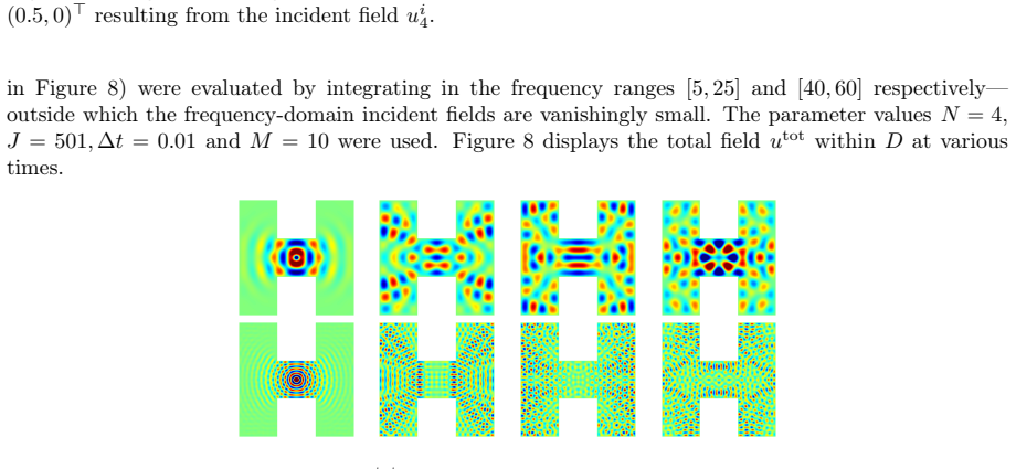
- The number of patches $N$ is a free parameter: the paper demonstrates $N = 3$ and $N = 6$ for a disk, $N = 4$ for an H-shaped cavity, and $N = 6$ and $N = 10$ for open-arc cavities, and shows that decomposing a trapping circular cavity into six patches reduces GMRES iteration counts.
- Because every patch solve within a scattering round is independent, the method parallelizes embarrassingly across patches and time windows; for non-trapping patches, Remark 3.7 argues that only finitely many multiple-scattering terms remain significant as $t$ grows, so the per-time cost stays bounded.
- The exterior version handles collections of closed curves and open arcs alike, including a highly trapping open circular cavity and a rocket-like open cavity, a capability the previous two-patch method lacked because its endpoint-singularity handling excluded open-arc scatterers.
Reading between the lines
- The paper does not draw the trade-off consequence of its own formula: since the exactness horizon per round is $\delta_{\min}/c$, the number of scattering rounds needed for a fixed final time is $cT/\delta_{\min}$, so choosing patch overlaps tunes the balance between the number of frequency-domain solves and the difficulty of each solve.
- The foundation is narrow in a specific way the authors acknowledge but do not quantify: Condition 2.3 is proven only for a flat arc, so the entire multi-patch identity currently rests on that single calculation plus curved-arc numerics; a counterexample search on a strongly concave or non-smooth arc would directly test the method's scope.
- The reduction to open-arc Helmholtz problems is not acoustic-specific: any linear wave phenomenon with finite propagation speed, a Fourier-reducible frequency problem, and uniquely solvable open-boundary integral equations fits the same template, which is the natural reading of the authors' stated plan to extend to elasticity, electromagnetics, and layered media.
- A separation the numerical section cannot itself establish is that the identity $u_M = u$ and the conjectured singularity form (4.7) are logically independent, so the observed accuracy of the solver is joint evidence for both; if (4.7) failed for some geometry, the scheme's high-order accuracy would break while the theorem could still hold.
Signed reviews
Editorial analysis
A structured set of objections, weighed in public.
Referee Report
Summary. This paper presents a multi-patch, multiple-scattering frequency-time hybrid (FTH-MS) integral equation method for the two-dimensional wave equation in interior and exterior domains. The boundary is partitioned into overlapping open arcs Γj with a smooth partition of unity; the Dirichlet problem is decomposed into a sequence of exterior open-arc wave problems, each solved in the frequency domain by uniquely solvable single-layer (or combined-field) integral equations. The main correctness result, Theorem 3.5, asserts that the M-th multiple-scattering sum u_M equals the exact solution u on D×(-∞,T(M)] with T(M)=M δ_min/c, provided the patches satisfy the conjectured restricted Huygens condition (Condition 2.3). The paper also describes a smoothing change of variables for endpoint and induced density singularities, discusses parallelization, and reports numerical experiments for discs, H-shaped cavities, multiple closed obstacles, open arcs, and highly trapping cavities.
Significance. If Condition 2.3 is granted, the paper provides a transparent reduction of trapped interior wave problems to a sequence of uniquely solvable open-arc Helmholtz problems. The induction proof of Lemma 3.4 and the boundary verification in Theorem 3.5 are clean and do not involve fitted parameters or circular normalizations; the method generalizes the earlier two-patch solver [22] to arbitrary patch numbers, handles open-arc scatterers, and is naturally parallel. The numerical examples are broad and support the claimed accuracy and long-time stability. The main limitation is that the central theoretical identity is conditional on an unproved conjecture (Condition 2.3), and the high-order numerical treatment relies on a conjectural singularity structure (4.7). These two points are the principal barriers to accepting the paper in its present form.
major comments (3)
- [Section 2.3, Lemma 3.1, Lemma 3.4, Theorem 3.5] Condition 2.3 is explicitly conjectural ('The proof is left for future work') and is assumed throughout the paper, yet it is load-bearing: Lemma 3.1 uses it to obtain (3.7), the inductive proof of Lemma 3.4 uses Lemma 3.1 to establish (3.18), and Theorem 3.5 uses those relations to verify the boundary condition (3.23). If Condition 2.3 fails for a curved or closed arc, the identity u=u_M on D×(-∞,T(M)] is not established. I therefore request that the manuscript either (a) prove Condition 2.3 for the classes of arcs used in Section 5, or (b) state Theorem 3.5 with Condition 2.3 as an explicit hypothesis and revise the concluding claim in Section 6 that the identity has been 'established rigorously' so that the conditional character is transparent. The induction argument itself appears sound conditional on this hypothesis.
- [Section 4.3] The change-of-variables (4.8) and the resulting claim of high-order accuracy for open-arc FTH-MS problems rest on the assertion (4.7) that every endpoint and induced singularity of the densities Ψj,m,q has the form f(d_p^{1/2})/d_p^{1/2} with f smooth. The paper states that this is preliminary analysis, that a proof is an open question, and that the only evidence is numerical smoothness of eΨj,m,q for one configuration. Since the CoV is used in all numerical examples of Section 5, the numerical accuracy claims are conditional on this unproved singularity structure. Please either prove (4.7) for the relevant settings or add resolution/convergence studies that directly confirm the predicted order for the actual FTH-MS densities, and state the assumption explicitly wherever the CoV is used.
- [Section 3.1 / Lemma 3.1] Lemma 3.1 is stated without proof, but it is the bridge between Condition 2.3 and the vanishing statements used in Lemma 3.4. Because Condition 2.3 is formulated with a time restriction t ≤ c^{-1} dist(Cinc,{e1,e2}), a time-shift argument is needed to obtain (3.7) for general T0. Please include a concise proof of Lemma 3.1 (or state it as following from the unrestricted form of Condition 2.3, if that is intended).
minor comments (6)
- [Abstract] Please fix 'arbitrary of number' in the abstract; it should read 'arbitrary number'.
- [Lemma 3.4] In the proof around (3.20), the notation v_{k,j,L} is used where the definition (3.12) gives ev_{k,j,L}; align the notation.
- [Figure 11] The caption refers to incident field u_i^1 but the text in Section 5 (Geometry 3) describes results for u_i^2; please correct.
- [Section 2.2] In the paragraph following (2.12), 'the time-domain solution U(x,t)' should be 'u(x,t)'.
- [Equation (4.7)] The display of (4.7) is difficult to read in the present formatting; please typeset the fraction properly and state explicitly that d_p(x) is the Euclidean distance from x to the endpoint p.
- [Section 3.3] The exterior extension is described as following with 'minimal modifications', but no formal analogue of Theorem 3.5 is stated for E=De; please state the exact multiple-scattering identity and its hypotheses for the exterior case, or explicitly mark it as a conjecture.
Circularity Check
No significant circularity: the FTH-MS sum identity follows from the recursive definitions and the explicit Huygens condition; the main caveat is the unproved, self-authored Condition 2.3, which is an explicit assumption rather than a fitted or self-referential input.
full rationale
The derivation chain is self-contained in the sense relevant to circularity. Definition 3.2 recursively builds the boundary data g_{j,m+1} from the previous open-arc iterates v_{k,m}; Lemma 3.4 proves the relations (3.16)-(3.18) by induction using only the partition-of-unity property (3.1)-(3.2), the boundary conditions (3.9), and the truncation rule (3.12). Theorem 3.5 combines these algebraic identities with Lemma 3.1, which is a geometric specialization of Condition 2.3, to verify the boundary equation (3.23); uniqueness of the interior wave-equation problem then gives (3.22). No parameter is fitted to the target solution, and the numerical accuracy claims are checked against exact solutions u=-u_i (Geometries 1 and 3) or independent fine-discretization references, so the predictions are not self-confirming. The only caveat touching the theorem's logical status is Condition 2.3 itself: Section 2.3 states that it is conjectural, was proved only for a flat arc, was numerically demonstrated for curved arcs in [22], and that 'throughout this paper Condition 2.3 is assumed to be valid.' This hypothesis is genuinely load-bearing, since Lemma 3.1, the inductive step (3.18), and the boundary verification (3.23) all use it. However, this is a correctness/rigor gap rather than circularity: the paper does not define the target solution in terms of the condition, does not fit u_M to u, and does not cite [22] as a proof of Condition 2.3—it explicitly labels the condition as an assumption. The central multiple-scattering algebra remains independent of any fitted or constructed input. Score 1 reflects the self-authored, conjectural nature of the unproved condition while the core derivation is not circular.
Assumptions & free parameters
assumptions (4)
- domain assumption Condition 2.3 (restricted Huygens domain-of-influence): for open/closed Lipschitz curves, solutions propagate along the boundary at sound speed, so data supported on Cinc produce zero field before t <= c^-1 dist(Cinc, endpoints).
- ad hoc to paper Singularity structure (4.7): all endpoint and induced endpoint singularities of open-arc densities take the form f(d_p^{1/2}) / d_p^{1/2} with f smooth.
- domain assumption Rapid decay of multiple-scattering iterates vj,m on non-trapping patches, keeping the number of active terms bounded as time grows.
- standard math Standard time-domain well-posedness and regularity of wave problems on closed curves and open arcs (Theorem 2.4).
Cite this review
Pith. "Pith review of Multi-patch/multiple-scattering frequency-time hybrid solver for interior and exterior wave equation problems." pith.science (2026). https://pith.science/paper/OUJ2KKOZ
@misc{pith2026250705725,
  author       = {Pith},
  title        = {Pith review of: Multi-patch/multiple-scattering frequency-time hybrid solver for interior and exterior wave equation problems},
  year         = {2026},
  howpublished = {\url{https://pith.science/paper/OUJ2KKOZ}},
  note         = {Machine review of arXiv:2507.05725}
}
read the original abstract
This paper proposes a new multiple-scattering frequency-time hybrid (FTH-MS) integral equation solver for problems of wave scattering by obstacles in two dimensional space, including interior problems in closed cavities and problems exterior to a set of disconnected open or closed scattering obstacles. The multiple-scattering FTH-MS method is based on a partition of the domain boundary into a user-prescribed set of overlapping open arcs, along with a corresponding sequence of multiple-scattering problems that effectively decompose the interior problem into a series of open-arc wave equation subproblems. The new strategy provides a significant extension of the original FTH-MS algorithm originally presented in [22], in that (1) By allowing for use of an arbitrary of number of component arcs, and not just two as in the previous contribution, the new approach affords (1a) A significantly increased geometric flexibility, as well as, (1b) The use of partitions for which each open arc leads to small numbers of iterations if iterative linear-algebra solvers are employed; and, (2) It facilitates parallelization -- as the subproblem solutions that are needed at each multiple scattering step can be evaluated in an embarrassingly parallel fashion. Utilizing a suitably-implemented Fourier transformation, each sub-problem is reduced to a Helmholtz frequency-domain problem that is tackled via a uniquely-solvable boundary integral equation. Similar FTH-MS methods are also presented for problems exterior to a number of bounded obstacles. All of the algorithms considered incorporate the previously introduced ``time-windowing and recentering'' methodology (that enables both treatment of incident signals of long duration and long time simulation), as well as a high-frequency Fourier transform algorithm that delivers numerically dispersionless, spectrally-accurate time evolution for arbitrarily long times.
Figures


Figures from the paper (14 more)




Forward citations
Cited by 1 Pith paper
-
Efficient time-domain scattering synthesis via frequency-domain singularity subtraction
A frequency-domain singularity subtraction technique, with real-frequency-only resonance identification via rational approximation, enables efficient long-time time-domain scattering simulations for trapping obstacles.
Reference graph
Works this paper leans on
-
[22]
O.P.Bruno, T.Yin, Multiple-scatteringfrequency-timehybridsolverforthewaveequationininterior domains, Math. Comput. 93(346) (2024) 551-587
work page 2024
-
[1]
A. Aimi, M. Diligenti, C. Guardasoni, On the energetic Galerkin boundary element method applied to interior wave propagation problems, J. Comput. Appl. Math. 235(7) (2011) 1746-1754
work page 2011
-
[2]
E. Akhmetgaliyev and O. Bruno, Regularized integral formulation of mixed Dirichlet-Neumann prob- lems, Journal of Integral Equations and applications 29 (2017) 493-529
work page 2017
- [3]
- [4]
-
[5]
"Bootstrap Domain of Dependence": Bounds and Time Decay of Solutions of the Wave Equation
T.G. Anderson and O. P. Bruno, “Bootstrap Domain of Dependence”: Bounds and Time Decay of Solutions of the Wave Equation, arXiv preprint arXiv:2010.09002 (2022)
work page Pith review arXiv 2022
-
[6]
T.G. Anderson, O. P. Bruno, M. Lyon, High-order, dispersionless “fast-hybrid” wave equation solver. Part I: O(1) sampling cost via incident-field windowing and recentering, SIAM J. Sci. Comput. 422 (2020) A1348-A1379
work page 2020
-
[7]
T.G.Anderson, O.P.Bruno, M.Lyon, FastHybridwaveequationsolverPartII:3Dwindowtracking, 2D asymptotics tracking, general incident fields and remote field evaluation, In preparation
Show all 51 references
-
[8]
Babuška, S.A
I.M. Babuška, S.A. Sauter, Is the pollution effect of the FEM avoidable for the Helmholtz equation considering high wave numbers? SIAM J. Numer. Anal. 34 (1997) 2392-2423. 25
1997
-
[9]
Bamberger, T
A. Bamberger, T. Ha-Duong, Formulation variationelle espace-temps pour le calcul par potentiel retardé de la diffraction d’une onde acoustique, Math. Methods Appl. Sci. 8 (1986) 405-435
1986
-
[10]
Banjai, M
L. Banjai, M. Kachanovska, Fast convolution quadrature for the wave equation in three dimensions, J. Comput. Phy. 279 (2014) 103-126
2014
-
[11]
Bansal, A
P. Bansal, A. Moiola, I. Perugia, C. Schwab, Space-time discontinuous Galerkin approximation of acoustic waves with point singularities, IMA J. Numer. Anal. 41 (2021) 2056-2109
2021
-
[12]
Barnett, L
A.H. Barnett, L. Greengard, T. Hagstrom, High-order discretization of a stable time-domain integral equation for 3D acoustic scattering, J. Comput. Phy. 402 (2020) 109047
2020
-
[13]
Interpolated Factored Green Function
C. Bauinger, O.P. Bruno, “Interpolated Factored Green Function” method for accelerated solution of scattering problems, J. Comput. Phy. 430 (2021) 110095
2021
-
[14]
Berenger, A perfectly matched layer for the absorption of electromagnetic waves, J
J.-P. Berenger, A perfectly matched layer for the absorption of electromagnetic waves, J. Comput. Phy. 114 (1994) 185-200
1994
-
[15]
Bruno, M
O.P. Bruno, M. Lyon, C. Pérez-Arancibia, C. Turc, Windowed Green function method for layered- media scattering, SIAM J. Appl. Math. 76(5) (2016) 1871-1898
2016
-
[16]
Bruno, E
O.P. Bruno, E. Garza, A Chebyshev-based rectangular-polar integral solver for scattering by general geometries described by non-overlapping patches, J. Comput. Phys. 421 (2020) 109740
2020
-
[17]
Bruno, E
O.P. Bruno, E. Garza, C. Pérez-Arancibia, Windowed Green function method for nonuniform open- waveguide problems, IEEE Trans. Antenn. Propag. 65 (2017) 4684-4692
2017
-
[18]
Bruno, S
O.P. Bruno, S. Lintner, Second-kind integral solvers for TE and TM problems of diffraction by open arcs, Radio Sci. 47 (6) (2012)
2012
-
[19]
Bruno, M
O.P. Bruno, M. Lyon, High-order unconditionally stable FC-AD solvers for general smooth domains I. Basic elements, J. Comput. Phys. 229 (6) (2010) 2009-2033
2010
-
[20]
Bruno, T
O.P. Bruno, T. Yin, Regularized integral equation methods for the elastic scattering problems in three dimensions, J. Comput. Phys. 410 (2020) 109350
2020
-
[21]
Bruno, T
O.P. Bruno, T. Yin, A windowed Green function method for elastic scattering problems on a half- space, Comput. Methods Appl. Mech. Engrg. 376 (2021) 113651
2021
-
[23]
Q. Chen, H. Haddar, A. Lechleiter, P. Monk, A sampling method for inverse scattering in the time domain, Inverse Problems 8 (2010) 85001-85017
2010
-
[24]
Colton and R
D. Colton and R. Kress, Inverse Acoustic and Electromagnetic Scattering Theory, Berlin, Springer, 1998
1998
-
[25]
Costabel, M
M. Costabel, M. Dauge, R. Duduchava, Asymptotics without logarithmic terms for crack problems, Commun. Partial Differ. Equ. 28 (2003) 869-926
2003
-
[26]
Douglas, J.E
J. Douglas, J.E. Santos, D. Sheen, L.S. Bennethum, Frequency domain treatment of one-dimensional scalar waves, Math. Models Methods Appl. Sci. 3 (1993) 171-194
1993
-
[27]
Ainsworth et al., eds., Springer Berlin Heidelberg, Berlin, Heidelberg, 2003, pp
T.Ha-Duong, Onretardedpotentialboundaryintegralequationsandtheirdiscretisation, inTopicsin Computational Wave Propagation: Direct and Inverse Problems, M. Ainsworth et al., eds., Springer Berlin Heidelberg, Berlin, Heidelberg, 2003, pp. 301–336. 26
2003
-
[28]
Engquist, A
B. Engquist, A. Majda, Absorbing boundary conditions for the numerical simulation of waves, Math. Comp. 31 (1977) 629–629
1977
-
[29]
Evans, Partial Differential Equations (2nd edition), Graduate Studies in Mathematics, Vol
L.C. Evans, Partial Differential Equations (2nd edition), Graduate Studies in Mathematics, Vol. 19, American Mathematical Society, Providence, 2010
2010
-
[30]
French, T.E
D.A. French, T.E. Peterson, A continuous space-time finite element method for the wave equation, Math. Comp. 65 (1996) 491-506
1996
-
[31]
Grote, A
M.J. Grote, A. Schneebeli, D. Schötzau, Dicontinuous Galerkin finite element method for the wave equation, SIAM J. Numer. Anal. 44 (2006) 2408-2431
2006
-
[32]
Hassell, T
M. Hassell, T. Qiu, T. Sánchez-Vizuet, F.-J. Sayas, A new and improved analysis of the time domain boundary integral operators for acoustics, J. Integral Equations Applications 29(1) (2017) 107-136
2017
-
[33]
Labarca, R
I. Labarca, R. Hiptmair, Acoustic scattering problems with convolution quadrature and the method of fundamental solutions, Commun. Comput. Phys. 30 (2021) 985-1008
2021
-
[34]
Laliena, F.-J
A.R. Laliena, F.-J. Sayas, Theoretical aspects of the application of convolution quadrature to scat- tering of acoustic waves, Numer. Math. 112 (2009) 637-678
2009
-
[35]
Liu, Fast Multipole Boundary Element Method, Cambridge University Press, New York, 2009
Y. Liu, Fast Multipole Boundary Element Method, Cambridge University Press, New York, 2009
2009
-
[36]
Löscher, O
R. Löscher, O. Steinbach, M. Zank, Numerical results for an unconditionally stable space-time finite element method for the wave equation, Domain Decomposition Methods in Science and Engineering XXVI, 625-632
-
[37]
Lubich, On the multistep time discretization of linear initial-boundary value problems and their boundary integral equations, Numer
C. Lubich, On the multistep time discretization of linear initial-boundary value problems and their boundary integral equations, Numer. Math. 67 (1994) 365-389
1994
-
[38]
R. C. MacCamy, Low frequency acoustic oscillations, Q. Appl. Math. 23 (1965) 247-255
1965
-
[39]
E.Mecocci, L.Misici, M.C.Recchioni, F.Zirilli, Anewformalismfortime-dependentwavescattering from a bounded obstacle, J. Acoust. Soc. Am. 107 (2000) 1825-1840
2000
-
[40]
J. M. Melenk and S. Sauter, Wavenumber explicit convergence analysis for galerkin discretizations of the helmholtz equation, SIAM J. Numer. Anal. 49 (2011) 1210–1243
2011
-
[41]
Sayas, Retarded Potentials andc Time Domain Boundary Integral Equations, Springer Inter- national Publishing, 2016
F.-J. Sayas, Retarded Potentials andc Time Domain Boundary Integral Equations, Springer Inter- national Publishing, 2016
2016
-
[42]
Shen and T
J. Shen and T. Tang, Spectral and High-Order Methods with Applications, Beijing Science Press, 2006
2006
-
[43]
Stephan, W.L
E.P. Stephan, W.L. Wendland, An augmented Galerkin procedure for the boundary integral method applied to two-dimensional screen and crack problems, Appl. Anal. 3 (1984) 183-219
1984
-
[44]
Steinbach, C
O. Steinbach, C. Urzúa-Torres, A new approach to space-time boundary integral equations for the wave equation, SIAM J. Math. Anal. 54(2) (2022) 1370-1392
2022
-
[45]
Steinbach, C
O. Steinbach, C. Urzúa-Torres, M. Zank, Towards coercive boundary element methods for the wave equation, arXiv:2106.01646
-
[46]
Stratton, Electromagnetic theory, McGraw-Hill, New York, 1941
J.A. Stratton, Electromagnetic theory, McGraw-Hill, New York, 1941
1941
-
[47]
Z. Sun, Y. Xing, Optimal error estimates of discontinuous Galerkin methods with generalized fluxes for wave equations on unstructured meshes, Math. Comput. 90 (2021) 1741-1772. 27
2021
-
[48]
Taflove, Computational electrodynamics: the finite-difference time-domain method, Artech House, Boston, 2000
A. Taflove, Computational electrodynamics: the finite-difference time-domain method, Artech House, Boston, 2000
2000
-
[49]
Werner, Low frequency asymptotics for the reduced wave equation in two-dimensional exterior spaces, Math
P. Werner, Low frequency asymptotics for the reduced wave equation in two-dimensional exterior spaces, Math. Meth. Appl. Sci. 8 (1986): 134-156
1986
-
[50]
Xing, C.-S
Y. Xing, C.-S. Chou, C.-W. Shu, Energy conserving local discontinuous Galerkin methods for wave propagation problems, Inverse Probl. Imag. 7 (2013) 967-986
2013
-
[51]
Y. Yue, F. Ma, B. Chen, Time domain linear sampling method for inverse scattering problems with cracks, E. Asian J. Appl. Math. 12(1) (2022) 96-110. 28
2022
Reviewed August 6, 2026 · model on record in the stance chip above.
Discussion (0). Continue with ORCID to comment.