A posteriori analysis of neural network approximations

Sergio Rojas; Thomas F\"uhrer

REVIEW 3 major objections 6 minor 32 references

A posteriori analysis of neural network approximations

T0 review · 3 major / 6 minor · reviewed 2026-08-06 · deepseek-v4-flash

Challenge this review Re-run · record.json Download PDF Read on arXiv ↗

Pith's one-line read For well-posed variational problems, any approximation's error is equivalent to the sum of two residuals; for elliptic equations both are computable.

desk verdict A solid generalization of the DPG a posteriori framework to neural network outputs, with a real practical contribution in the eta+rho loss, but the proven upper-bound guarantee only holds for exact quadrature while the computed estimators show a large quadrature gap. read the letter →

arxiv 2507.06017 v1 pith:NPJSTJXT submitted 2025-07-08 math.NA cs.NA

Thomas Führer , Sergio Rojas This is my paper · ORCID

classification math.NAcs.NA MSC 65N1565M6065M75

keywords aposteriorierrorestimationneuralnetworkapproximationsecond-orderellipticPDEresidualminimizationvariationalformulationadaptivemeshrefinementquadraturePhysics-InformedNetworks

verification ladder T0 review T1 audit T2 compute T3 formal

The pith

A machine-rendered reading of the paper's core claim, the machinery that carries it, and where it could break.

The reading

This paper works in a general Hilbert-space setting where the true solution u of a variational problem satisfies B u = F, and asks whether the error of an arbitrary approximation w, such as the output of a neural network, can be measured without knowing u. The answer is a two-term equivalence: the error is comparable to $\eta(w) + \mu(w)$, where $\eta(w)$ is the residual tested against a finite-dimensional space and therefore computable, while $\mu(w)$ is an infinite-dimensional remainder. For a diffusion-advection-reaction model problem, the paper shows how to bound $\mu(w)$ by a computable mesh-size-weighted estimator $\rho(w)$, so the $H^1$ error is controlled by $\eta(w)+\rho(w)$. That makes error monitoring and loss design possible: either track the two terms during training or put $\eta^2+\rho^2$ into the loss, and the numerical experiments indicate that including $\rho$ avoids the stagnation seen with $\eta$ alone.

What carries the argument

The engine is the pair $(\eta(w), \mu(w))$ defined in Section 2: $\eta(w) = \sup_{0 \ne v \in V_h} b(u-w,v)/\|v\|_{V_h}$ is the discrete MINRES-style residual, a computable lower bound; $\mu(w) = \sup_{0 \ne v \in V} b(w-u, v-\Pi_h v)/\|v\|_V$ is the part of the residual invisible to the finite-dimensional test space. The localization step replaces the abstract $\mu$ by the computable estimator $\rho(w)$, assembled from $L^2$ residuals inside elements, jumps of $A\nabla w$ across faces, and boundary contributions; Theorem 1 plus the bound $\mu(w) \le C\rho(w)$ turns the abstract equivalence into $\|u-w\|_{H^1(\Omega)} \simeq \eta(w)+\rho(w)$ for the elliptic model problems.

What would settle it

Decisive experiment: for a Poisson problem with known solution, train a smooth tanh network using only $\eta^2$ until $\eta$ is far below the true $H^1$ error, then compute the ratio $(\eta+\rho)/\|u-w\|_{H^1(\Omega)}$ along the trajectory and on uniformly refined meshes; the claimed equivalence predicts the ratio stays in a fixed interval independent of mesh and training state, while the paper's own Section 5.3 shows the ratio for $\eta$ alone drifts, so an unbounded drift in the $\eta+\rho$ ratio would falsify the theorem rather than the quadrature.

Watch

Extended reading notes

Core claim

The central result, Theorem 1, states that for any $w \in U$, $C_{\mathrm{equiv}}^{-1} \eta(w) \le \|B(u-w)\|_{V'} \le C_{\mathrm{equiv}}\|\Pi_h\|\eta(w) + \mu(w)$, and $\mu(w) \le \|1-\Pi_h\|\inf_{w_0 \in U_0(\Pi_h)} \|B(u-w-w_0)\|_{V'}$; when $B$ is bounded below, this yields $\|u-w\|_U \simeq \eta(w)+\mu(w)$ for every $w$. For the second-order elliptic model problem, the paper constructs a computable $\rho(w)$ from elementwise volume residuals, inter-element flux jumps, and boundary terms, proves $\mu(w) \le C\rho(w)$, and obtains the equivalence $\|u-w\|_{H^1(\Omega)} \simeq \eta(w)+\rho(w)$ in the weak, bubble-enriched, broken, and strong formulations (Theorems 14, 17, 19, 23). The claim is that, for any sufficiently smooth network output, the $H^1$ error is monitored and controlled by two terms that can be evaluated from $w$, the data, and the mesh alone.

Load-bearing premise

Everything rests on the network output being regular enough that elementwise residuals and inter-element jumps are well defined, which excludes ReLU activations, and on the second residual being bounded by the computable estimator up to a generic constant that the paper does not quantify.

Editorial extensions

If this is right

During optimization, the two computable terms give an online guarantee: the $H^1$ error of the current network output stays within fixed constants of $\eta(w)+\rho(w)$, so training can be stopped or adapted based on a trustworthy error proxy.
Using only $\eta^2$ as the loss can be misleading because $\eta$ can keep decreasing while the true error plateaus; adding $\rho^2$ restores the equivalence and yields a more robust loss (Section 5.3).
Dirichlet boundary conditions can be imposed weakly through boundary estimators rather than by architectural multiplication, and the experiments with a boundary layer show weak imposition learns much faster than strong enforcement (Section 5.4).
Quadrature errors can invalidate the estimator, and the paper's adaptive algorithm (Algorithm 1) detects the mismatch by comparing two quadrature rules and refining the mesh locally, which is essential for problems with singular gradients (Section 5.6).
The abstract theorem extends the same two-term error decomposition to any well-posed variational problem for which a bounded projection onto finite-dimensional test spaces and a localization of $\mu$ exist.

Reading between the lines

Editorial extensions of the paper, not claims the author makes directly.

The same certification pattern should transfer to other scientific machine-learning losses that are discrete dual norms, such as VPINN-type or least-squares losses: the missing ingredient is always the localization term $\rho$, and this construction suggests where to look for it.
Because the estimators depend on the function class only through smoothness and boundary regularity, any parameterized function family with the same differentiability, such as Fourier features or spline networks, could be certified by the same formulas.
A testable extension would treat the internal interfaces generated by ReLU-like activations as additional element boundaries, with jumps across those interfaces entering $\rho$; if accurate, this would remove the smoothness restriction the authors flag in Section 6.
The generic constant in the bound $\mu(w) \le C\rho(w)$ is left unquantified; a calibration of $C$ on manufactured solutions could turn the guarantee into a quantitative confidence interval for a given network and mesh, at the price of losing the a priori character.

Share X Bluesky LinkedIn Reddit HN

Editorial analysis

A structured set of objections, weighed in public.

Desk editor's note, referee report, and a circularity audit.

Desk Editor's Note

read the letter

Quick summary: this is a genuinely useful generalization of the DPG a posteriori framework to arbitrary trial functions, and the eta+rho loss is a real improvement over eta-only losses like RVPINN. The abstract machinery checks out; the soft spot is the quadrature gap between the theorems and the implemented quantities.

What is new: Theorem 1 replaces the finite-dimensional trial space assumption in [CDG14, Theorem 2.1] with arbitrary w in U, and the paper constructs concrete computable rho for several variational formulations of a second-order elliptic problem. The numerical section shows that training with eta^2+rho^2 outperforms eta^2 alone and classical PINN, and the boundary-layer experiment makes a fair point about weak enforcement of Dirichlet conditions. No fitted constants, no circularity; the estimates are derived from first principles and tested on manufactured solutions.

Soft spots, in order of size. The central practical claim is that eta+rho can monitor and control the H^1 error of a network output. As stated in Theorems 14/17/19/23, that claim requires exact quadrature. The paper mentions 'sufficiently accurate quadrature' once, but Sections 5.5 and 5.6 show this is not a minor technicality: with the fixed 6-point rule on the L-shaped singular example, the computed ratio Lwb/||u-u_theta|| falls to about 0.01, meaning the estimator badly underestimates the true error. Algorithm 1 is a heuristic discrepancy check; there is no proof that the refined mesh restores the upper bound, and the quadrature error inside the Riesz system for eta is not analyzed. So the proven upper-bound property applies to the exact-integral quantity, not to the quantity actually computed. That gap should be fixed or explicitly downgraded before publication.

Smaller issues: Lemma 8's operator construction is sketched and Lemma 10's proof is omitted, so a referee should check those. The equivalence constants are not quantified, which matters if the goal is 'guaranteed' control. The smoothness assumption excludes ReLU, and the paper says so honestly. The experiments are single-run, and no code is released; for a numerical paper that proposes a training loss, code and seed variance are relevant.

Who this is for: people working on neural PDE solvers, especially PINN/RVPINN variants, and anyone who wants a posteriori control in that setting. The framework is solid enough that I'd send it to a serious referee, but the referee should push on the quadrature gap and code availability. My verdict: accept for peer review, conditional on the authors either closing or clearly restating the quadrature assumption and releasing code and data.

Referee Report

3 major / 6 minor

Summary. The paper develops an abstract a posteriori error estimation framework for approximations that are not necessarily finite-element functions, with neural network outputs as the motivating application. Theorem 1 shows that, for a well-posed variational operator B: U -> V', the residual norm ||B(u-w)||_{V'} is bounded below by a computable discrete residual eta(w) and above by C||Pi_h|| eta(w) + mu(w), where mu(w) is a remainder term; when B is bounded below, ||u-w||_U is equivalent to eta(w)+mu(w). For a second-order elliptic model problem, the authors construct computable local estimators rho(w) that bound mu(w) for three variational formulations (weak, broken, strong) and for three boundary-condition treatments. The resulting theorems (Theorems 14, 17, 19, 23) give two-sided estimates eta(w) <~ ||u-w||_{H^1} <~ eta(w)+rho(w) under elementwise regularity assumptions and exact quadrature. The numerical section compares losses based on eta^2+rho^2 with classical PINN losses, studies boundary-condition enforcement, and proposes an adaptive mesh/quadrature refinement algorithm (Algorithm 1) to keep the ratio of the computed loss to the exact error under control in singular problems.

Significance. The abstract framework is clean and connects neural-network residual minimization with established MINRES/DPG a posteriori theory. The decomposition into a computable discrete residual eta and a localized upper bound rho is natural, and the paper gives a useful comparison of several variational formulations and boundary treatments. The estimators contain no fitted parameters, and the numerical validation uses manufactured and singular solutions. The authors also state the main limitations honestly, including the smoothness restriction that excludes ReLU activations (Section 6) and the dependence on quadrature. If the quadrature gap is closed or explicitly scoped, and the boundary lemmas are fully proven, the framework could be a solid basis for reliable loss construction for smooth-activation neural networks. As it stands, the central practical guarantee is proven only for exactly integrated residuals, and the experiments show that the computed estimators can deviate from the true error by orders of magnitude.

major comments (3)

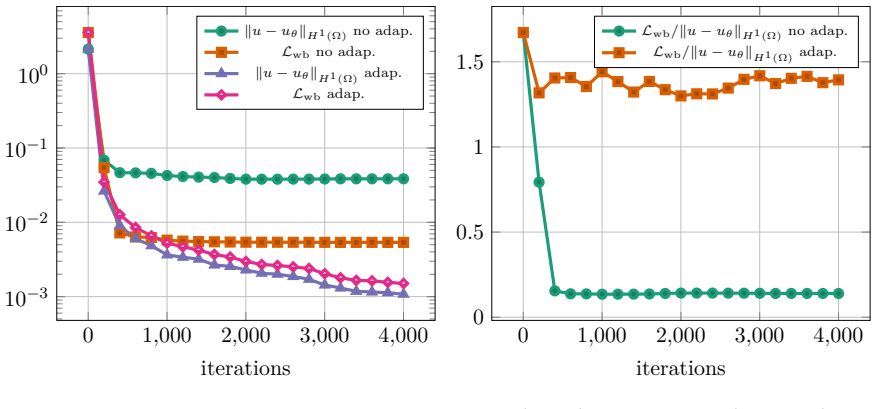
[Section 5.5, Section 5.6; Theorems 14, 17, 19, 23] The four main theorems are statements about the exact integrals defining eta and rho, but the practical claim concerns the quadrature-based implementation. The experiments in Section 5.5 and Section 5.6 show this distinction is not benign: with the fixed 6-point volume rule, the ratio Lwb/||u-u_theta||_{H^1} in the L-shaped singular example deteriorates to about 0.01 (Figure 5, 'no adap.'), meaning the computed estimator underestimates the true error by two orders of magnitude. Algorithm 1 is a heuristic discrepancy check between a low-order and a high-order quadrature rule; no theorem quantifies the quadrature perturbation of eta and rho, no analysis is given of the quadrature error in the discrete Riesz system (8) used to evaluate eta, and no proof is supplied that the marked-refinement loop restores the upper bound of Theorem 1. Since the stated purpose (Introduction, Section 5.5) is guaranteed monitoring and loss construction, the manuscript must either provide a rigorous quadrature-perturbation analysis and a guarantee for Algorithm 1, or explicitly restrict the guaranteed-control statements to exactly integrated residuals and present the numerical sections as heuristic evidence.
[Lemma 8 and Lemma 10] The proofs of the boundary lemmas are incomplete. In Lemma 8, the operator Pi_T is only sketched: the existence of the H(div) extension tau-tilde with the prescribed normal trace is asserted, the claimed range property of the dual operator (J_F^p)' is not demonstrated, the boundedness chain is compressed, and the case p=0 is dismissed as 'slightly more technical' without details. Lemma 10 is explicitly not proven ('We omit further details'). These lemmas establish the boundary inequality (13) that enters every main theorem through eta_Gamma and rho_Gamma, so the proofs need to be completed or replaced by a precise reference.
[Section 4.2, Eq. (17b); Theorems 14 and 17] The regularity assumption does not justify the jump term in rho_Omega. Theorems 14 and 17 assume only w in H^1(Omega) with div(A grad w)|_T in L^2(T) for each T; under this assumption the normal trace A grad w . n on inter-element facets is only in H^{-1/2}(dT), not in L^2(dT), so the term h_T ||[A grad w . n]||^2_{dT\Gamma} in (17b) and (19b) is not well defined, and the Cauchy-Schwarz estimate in the proof of Theorem 14 is not justified. The assumption should be strengthened (for example to w|_T in H^2(T), or to A grad w in H(div;Omega) with L^2 normal traces), or the jump term must be reformulated in the correct distributional setting.

minor comments (6)

[Corollary 4] The formula for C2 should involve a maximum, not a minimum, of C_{equiv,j}||Pi_{h,j}||; as written, the stated constant does not follow from the displayed calculation.
[Abstract and Section 2.1] The wording 'error is equivalent to the sum of two residuals' is stronger than what Theorems 14-23 prove; those theorems give eta <~ error <~ eta+rho, and Section 2.1 itself notes that rho need not be a lower bound for the error. Please align the abstract and concluding wording with the actual two-sided statements.
[Section 3.2.2, Lemma 8, Eqs. (14)-(16)] The degree indices of the boundary Scott-Zhang operator are inconsistent: Section 3.2.2 defines J_F^{p+1}, while Lemma 8 and Eqs. (14)-(16) use J_F^p. Please check and unify the notation.
[Section 5.5, Algorithm 1] In Algorithm 1, the symbol M is used both for the maximal local error (line 5) and for the marked set (lines 6-7); using distinct names would remove ambiguity.
[References] The arXiv identifier for [MSS24a] is listed as 2412.059965; this appears to be a typo for 2412.05996. Please correct.
[Section 2.1, Eq. (7); Theorems 14-23] The constants in (7) and in the 'less than or similar' relations of Theorems 14-23 are not quantified; the paper should state explicitly that they depend on shape regularity, the PDE coefficients, C_equiv, and the polynomial degrees, so that readers understand that the two-sided bound is qualitative rather than a computable constant-tight estimate.

Circularity Check

0 steps flagged · score 0.0 of 10

No significant circularity: the error equivalence and the computable upper bounds are derived from first principles with no fitted parameters or load-bearing self-citations.

full rationale

The derivation is self-contained. Theorem 1 proves the two-sided estimate in a purely Hilbert-space setting directly from the definitions of η(w), µ(w), and Π_h, together with the norm-equivalence assumption; the constants involve only C_equiv and ||Π_h||, and no fitted parameter enters. The Section 4 estimators (Theorems 14, 17, 19, and 23) bound µ by ρ through integration by parts, trace duality (Lemmas 5 and 7), and approximation properties of quasi-interpolators (Scott–Zhang and H(div)-stable projectors); these are standard external tools, not restatements of the paper's target results. The boundary estimators likewise follow from bounded projections cited from [AFK+13] and trace results from [CDG16]. The abstract caveat 'assuming sufficiently accurate quadrature' and the Section 6 admission that the assumptions exclude ReLU activations are explicit limitations of scope, not backwards definitions or hidden fits. Self-citations such as [RMMnM+24] for the observation that η alone can stagnate and [Füh21] for an H^{-1/2} norm equivalence are motivational or technical and are not load-bearing: the stagnation phenomenon is also demonstrated independently in the paper's own Figure 2, and the technical lemma supports efficient computation rather than the central equivalence. The numerical experiments against manufactured and singular solutions provide external benchmarks. The reviewer/skeptic concern about quadrature is a soundness and accuracy gap between the implemented estimator and the exactly integrated idealization, not a circularity, since the theorems explicitly state the exact-integration setting in which the estimates hold.

Assumptions & free parameters 1 free parameters · 5 assumptions · 0 invented entities

No fitted parameters enter the theoretical bounds; the only hand-chosen numbers are the mesh-refinement thresholds in Algorithm 1, which affect the experiments but not the error equivalence. No new physical or mathematical entities are postulated.

free parameters (1)

Marking thresholds tau1, tau2 in Algorithm 1 = tau1=0.3, tau2=0.7 (Section 5.5); tau1=0.2, tau2=0.75 (Section 5.6)
Hand-chosen adaptivity parameters controlling when to refine the mesh; they influence the numerical results but are not part of the theoretical error equivalence.

assumptions (5)

domain assumption Well-posedness of the model problem: A uniformly elliptic, beta in L^infinity, c in L^infinity with -1/2 div beta + c >= 0, f in H^{-1}(Omega), g in H^{1/2}(Gamma).
Section 4: ensures existence, uniqueness, and the norm equivalence used throughout.
standard math Trace duality identities for H^{1/2}(Gamma) and H^{-1/2}(Gamma) (Lemma 5).
Section 3.1: invoked to relate boundary residual norms to H(div) and fractional trace spaces; proof from [CDG16, Lemma 2.2].
standard math Standard approximation and stability properties of Scott-Zhang type operators and the commuting H(div) interpolant from [EGSV22].
Section 3.2: used to localize mu and bound rho; the exact constants and trace behavior of the operator in Lemma 8 are only sketched.
domain assumption Sufficient smoothness of the approximation: div A grad w|_T in L^2(T) and w|_Gamma in H^1(Gamma).
Section 4 and Section 6: required for rho_Omega (volume jumps) and rho_Gamma to be well defined; excludes ReLU activations.
domain assumption Quadrature is accurate enough that numerical evaluation of eta and rho approximates the exact norms.
Abstract and Section 5.5: the adaptive algorithm assumes a discrepancy between L and L_hat diagnoses integration error; otherwise the computed loss is not a faithful estimator.

how reviews work

0 comments

Cite this review

Pith. "Pith review of A posteriori analysis of neural network approximations." pith.science (2026). https://pith.science/paper/NPJSTJXT

@misc{pith2026250706017,
  author       = {Pith},
  title        = {Pith review of: A posteriori analysis of neural network approximations},
  year         = {2026},
  howpublished = {\url{https://pith.science/paper/NPJSTJXT}},
  note         = {Machine review of arXiv:2507.06017}
}

read the original abstract

In a general setting, we study a posteriori estimates used in finite element analysis to measure the error between a solution and its approximation. The latter is not necessarily generated by a finite element method. We show that the error is equivalent to the sum of two residuals provided that the underlying variational formulation is well posed. The first contribution is the projection of the residual to a finite-dimensional space and is therefore computable, while the second one can be reliably estimated by a computable upper bound in many practical scenarios. Assuming sufficiently accurate quadrature, our findings can be used to estimate the error of, e.g., neural network outputs. Two important applications can be considered during optimization: first, the estimators are used to monitor the error in each solver step, or, second, the two estimators are included in the loss functional, and therefore provide control over the error. As a model problem, we consider a second-order elliptic partial differential equation and discuss different variational formulations thereof, including several options to include boundary conditions in the estimators. Various numerical experiments are presented to validate our findings.

Figures

Figures reproduced from arXiv: 2507.06017 by the authors.

**Figure 1.** First row shows error in H1 (Ω) norm over time (left) and number of iterations (right). The second row shows the ratio between the square root of the loss and the error in the energy norm. 5.5. Effect of quadrature and adaptive algorithm. For this experiment we study quadrature and how to locally refine the mesh in order to increase the number of quadrature points in a specific region. On an element T ∈ T we use, as… view at source ↗

**Figure 2.** The left plot shows H1 (Ω) norm over number of iterations (epochs). The right plot shows the ratio between the square root of the loss and the error in the energy norm. 0 0.2 0.4 0.6 0.8 1 0 0.2 0.4 0.6 0.8 1 0 500 1,000 1,500 2,000 2,500 3,000 10−2 10−1 100 iterations enforcing bc not enforcing bc [PITH_FULL_IMAGE:figures/full_fig_p021_2.png] view at source ↗

**Figure 3.** Comparing the inclusion of “enforcing boundary conditions” by multiplying network output with φ (Section 5.4). we note that there exists unique discrete functions rΩ ∈ VΩ,T ⊂ H1 0 (Ω), rΓ ∈ VΓ,T ⊂ H(div; Ω) with η 2 Ω = ∥∇rΩ∥ 2 Ω, η2 Γ = ∥rΓ∥ 2 H(div;Ω) which can then be decomposed into local contributions. To compute Lwb we use quadrature QT ,F and define Lbwb analogously but using the higher order quadrature QbT … view at source ↗

Figures from the paper (2 more)

**Figure 4.** Figure 4: Results for setup of Section 5.5 with (adap.) and without (no adap.) using Algorithm 1. nodes in Ω and 256 quadrature nodes on Γ (labeled no adap.). One observes the loss of robustness without using Algorithm 1 although the total number of quadrature nodes is larger. I…

**Figure 5.** Figure 5: Results for problem on L-shaped domain with singular solution (Section 5.6). [BCPS23] Stefano Berrone, Claudio Canuto, Moreno Pintore, and Natarajan Sukumar. Enforcing dirichlet boundary conditions in physics-informed neural networks and variational physics-informed ne…

Discussion (0). Continue with ORCID to comment.

Reference graph

Works this paper leans on

32 extracted references · 29 canonical work pages

[1]

Aurada, M

M. Aurada, M. Feischl, J. Kemetm\"uller, M. Page, and D. Praetorius. Each H^ 1/2 -stable projection yields convergence and quasi-optimality of adaptive FEM with inhomogeneous D irichlet data in R^d . ESAIM Math. Model. Numer. Anal. , 47(4):1207--1235, 2013

work page 2013
[2]

Enforcing dirichlet boundary conditions in physics-informed neural networks and variational physics-informed neural networks

Stefano Berrone, Claudio Canuto, Moreno Pintore, and Natarajan Sukumar. Enforcing dirichlet boundary conditions in physics-informed neural networks and variational physics-informed neural networks. Heliyon , 9(8), 2023

work page 2023
[3]

Bochev and Max D

Pavel B. Bochev and Max D. Gunzburger. Least-squares finite element methods , volume 166 of Applied Mathematical Sciences . Springer, New York, 2009

work page 2009
[4]

Finite element interpolated neural networks for solving forward and inverse problems

Santiago Badia, Wei Li, and Alberto F Mart \' n. Finite element interpolated neural networks for solving forward and inverse problems. Computer Methods in Applied Mechanics and Engineering , 418:116505, 2024

work page 2024
[5]

Numerical solution of inverse problems by weak adversarial networks

Gang Bao, Xiaojing Ye, Yaohua Zang, and Haomin Zhou. Numerical solution of inverse problems by weak adversarial networks. Inverse Problems , 36(11):115003, 31, 2020

work page 2020
[6]

Deep least-squares methods: An unsupervised learning-based numerical method for solving elliptic pdes

Zhiqiang Cai, Jingshuang Chen, Min Liu, and Xinyu Liu. Deep least-squares methods: An unsupervised learning-based numerical method for solving elliptic pdes. Journal of Computational Physics , 420:109707, 2020

work page 2020
[7]

A posteriori error control for DPG methods

Carsten Carstensen, Leszek Demkowicz, and Jay Gopalakrishnan. A posteriori error control for DPG methods. SIAM J. Numer. Anal. , 52(3):1335--1353, 2014

work page 2014
[8]

Carstensen, L

C. Carstensen, L. Demkowicz, and J. Gopalakrishnan. Breaking spaces and forms for the DPG method and applications including M axwell equations. Comput. Math. Appl. , 72(3):494--522, 2016

work page 2016

Show all 32 references

[9]

Demkowicz and J

L. Demkowicz and J. Gopalakrishnan. A primal DPG method without a first-order reformulation. Comput. Math. Appl. , 66(6):1058--1064, 2013

2013
[10]

The discontinuous petrov–galerkin method

Leszek Demkowicz and Jay Gopalakrishnan. The discontinuous petrov–galerkin method. Acta Numerica , 34:293–384, 2025

2025
[11]

Equivalence of local- and global-best approximations, a simple stable local commuting projector, and optimal hp approximation estimates in H( div )

Alexandre Ern, Thirupathi Gudi, Iain Smears, and Martin Vohral\'ik. Equivalence of local- and global-best approximations, a simple stable local commuting projector, and optimal hp approximation estimates in H( div ) . IMA J. Numer. Anal. , 42(2):1023--1049, 2022

2022
[12]

A posteriori certification for physics-informed neural networks

Lewin Ernst, Nikolaos Rekatsinas, and Karsten Urban. A posteriori certification for physics-informed neural networks. arXiv preprint arXiv:2502.20336 , 2025

2025 arXiv
[13]

Multilevel decompositions and norms for negative order S obolev spaces

Thomas F \"u hrer. Multilevel decompositions and norms for negative order S obolev spaces. Math. Comp. , 91(333):183--218, 2021

2021
[14]

Hiptmair

R. Hiptmair. Multigrid method for H( div ) in three dimensions. volume 6, pages 133--152. 1997. Special issue on multilevel methods (Copper Mountain, CO, 1997)

1997
[15]

Characterizing possible failure modes in physics-informed neural networks

Aditi Krishnapriyan, Amir Gholami, Shandian Zhe, Robert Kirby, and Michael W Mahoney. Characterizing possible failure modes in physics-informed neural networks. Advances in Neural Information Processing Systems , 34:26548--26560, 2021

2021
[16]

Variational physics-informed neural networks for solving partial differential equations

Ehsan Kharazmi, Zhongqiang Zhang, and George Em Karniadakis. Variational physics-informed neural networks for solving partial differential equations. arXiv preprint arXiv:1912.00873 , 2019

1912 arXiv
[17]

hp-vpinns: Variational physics-informed neural networks with domain decomposition

Ehsan Kharazmi, Zhongqiang Zhang, and George Em Karniadakis. hp-vpinns: Variational physics-informed neural networks with domain decomposition. Computer Methods in Applied Mechanics and Engineering , 374:113547, 2021

2021
[18]

Deep learning

Yann LeCun, Yoshua Bengio, and Geoffrey Hinton. Deep learning. nature , 521(7553):436--444, 2015

2015
[19]

Quasi-optimal least squares: Inhomogeneous boundary conditions, and application with machine learning

Harald Monsuur, Robin Smeets, and Rob Stevenson. Quasi-optimal least squares: Inhomogeneous boundary conditions, and application with machine learning. arXiv preprint arXiv:2412.059965 , 2024

2024 arXiv
[20]

Minimal residual methods in negative or fractional S obolev norms

Harald Monsuur, Rob Stevenson, and Johannes Storn. Minimal residual methods in negative or fractional S obolev norms. Math. Comp. , 93(347):1027--1052, 2024

2024
[21]

Multilevel finite element approximation

Peter Oswald. Multilevel finite element approximation . Teubner Skripten zur Numerik. [Teubner Scripts on Numerical Mathematics]. B. G. Teubner, Stuttgart, 1994. Theory and applications

1994
[22]

Robust variational physics-informed neural networks

Sergio Rojas, Pawe Maczuga, Judit Mu\ noz Matute, David Pardo, and Maciej Paszy\'nski. Robust variational physics-informed neural networks. Comput. Methods Appl. Mech. Engrg. , 425:Paper No. 116904, 18, 2024

2024
[23]

Physics-informed neural networks: A deep learning framework for solving forward and inverse problems involving nonlinear partial differential equations

Maziar Raissi, Paris Perdikaris, and George E Karniadakis. Physics-informed neural networks: A deep learning framework for solving forward and inverse problems involving nonlinear partial differential equations. Journal of Computational physics , 378:686--707, 2019

2019
[24]

Stephan and Thanh Tran

Ernst P. Stephan and Thanh Tran. Schwarz methods and multilevel preconditioners for boundary element methods . Springer, Cham, [2021] 2021

2021
[25]

Uniform preconditioners for problems of negative order

Rob Stevenson and Raymond van Veneti\"e. Uniform preconditioners for problems of negative order. Math. Comp. , 89(322):645--674, 2020

2020
[26]

Uniform preconditioners for problems of positive order

Rob Stevenson and Raymond van Veneti\"e. Uniform preconditioners for problems of positive order. Comput. Math. Appl. , 79(12):3516--3530, 2020

2020
[27]

A deep fourier residual method for solving pdes using neural networks

Jamie M Taylor, David Pardo, and Ignacio Muga. A deep fourier residual method for solving pdes using neural networks. Computer Methods in Applied Mechanics and Engineering , 405:115850, 2023

2023
[28]

Optimizing variational physics-informed neural networks using least squares

Carlos Uriarte, Manuela Bastidas, David Pardo, Jamie M Taylor, and Sergio Rojas. Optimizing variational physics-informed neural networks using least squares. Computers & Mathematics with Applications , 185:76--93, 2025

2025
[29]

Neural network methods for power series problems of perron-frobenius operators

Tanakorn Udomworarat, Ignacio Brevis, Martin Richter, Sergio Rojas, and Kristoffer G van der Zee. Neural network methods for power series problems of perron-frobenius operators. arXiv preprint arXiv:2505.05407 , 2025

2025
[30]

Verf\"urth

R. Verf\"urth. A posteriori error estimation and adaptive mesh-refinement techniques. In Proceedings of the F ifth I nternational C ongress on C omputational and A pplied M athematics ( L euven, 1992) , volume 50, pages 67--83, 1994

1992
[31]

When and why pinns fail to train: A neural tangent kernel perspective

Sifan Wang, Xinling Yu, and Paris Perdikaris. When and why pinns fail to train: A neural tangent kernel perspective. Journal of Computational Physics , 449:110768, 2022

2022
[32]

The deep ritz method: a deep learning-based numerical algorithm for solving variational problems

Bing Yu et al. The deep ritz method: a deep learning-based numerical algorithm for solving variational problems. Communications in Mathematics and Statistics , 6(1):1--12, 2018

2018

Pith tools

Reviewed August 6, 2026 · model on record in the stance chip above.

[1] [1]

Aurada, M

M. Aurada, M. Feischl, J. Kemetm\"uller, M. Page, and D. Praetorius. Each H^ 1/2 -stable projection yields convergence and quasi-optimality of adaptive FEM with inhomogeneous D irichlet data in R^d . ESAIM Math. Model. Numer. Anal. , 47(4):1207--1235, 2013

work page 2013

[2] [2]

Enforcing dirichlet boundary conditions in physics-informed neural networks and variational physics-informed neural networks

Stefano Berrone, Claudio Canuto, Moreno Pintore, and Natarajan Sukumar. Enforcing dirichlet boundary conditions in physics-informed neural networks and variational physics-informed neural networks. Heliyon , 9(8), 2023

work page 2023

[3] [3]

Bochev and Max D

Pavel B. Bochev and Max D. Gunzburger. Least-squares finite element methods , volume 166 of Applied Mathematical Sciences . Springer, New York, 2009

work page 2009

[4] [4]

Finite element interpolated neural networks for solving forward and inverse problems

Santiago Badia, Wei Li, and Alberto F Mart \' n. Finite element interpolated neural networks for solving forward and inverse problems. Computer Methods in Applied Mechanics and Engineering , 418:116505, 2024

work page 2024

[5] [5]

Numerical solution of inverse problems by weak adversarial networks

Gang Bao, Xiaojing Ye, Yaohua Zang, and Haomin Zhou. Numerical solution of inverse problems by weak adversarial networks. Inverse Problems , 36(11):115003, 31, 2020

work page 2020

[6] [6]

Deep least-squares methods: An unsupervised learning-based numerical method for solving elliptic pdes

Zhiqiang Cai, Jingshuang Chen, Min Liu, and Xinyu Liu. Deep least-squares methods: An unsupervised learning-based numerical method for solving elliptic pdes. Journal of Computational Physics , 420:109707, 2020

work page 2020

[7] [7]

A posteriori error control for DPG methods

Carsten Carstensen, Leszek Demkowicz, and Jay Gopalakrishnan. A posteriori error control for DPG methods. SIAM J. Numer. Anal. , 52(3):1335--1353, 2014

work page 2014

[8] [8]

Carstensen, L

C. Carstensen, L. Demkowicz, and J. Gopalakrishnan. Breaking spaces and forms for the DPG method and applications including M axwell equations. Comput. Math. Appl. , 72(3):494--522, 2016

work page 2016