REVIEW 4 major objections 6 minor 1 cited by
A three-step approach to reliably estimate magnetic field strengths in star-forming regions
T0 review · 4 major / 6 minor · reviewed 2026-08-06 · deepseek-v4-flash
Pith's one-line read A three-step measurement recipe—radiative-transfer density, second-moment velocity dispersion, and Gaussian-deconvolved polarization angles—makes the ST estimator recover plane-of-sky magnetic field strength in star-forming clouds within…
desk verdict A well-executed single-simulation calibration study with a useful recipe, but the generality claim is in-sample; the paper deserves review but needs an out-of-sample test. read the letter →
The pith
A machine-rendered reading of the paper's core claim, the machinery that carries it, and where it could break.
The reading
What carries the argument
The load-bearing object is the corrected parameter triple entering two energy-equipartition estimators: the classic DCF relation $B_{\rm POS}=f\sqrt{4\pi\rho}\,\delta v/\delta\theta$ and the ST relation $B_{\rm POS}=\sqrt{2\pi\rho}\,\delta v/\sqrt{\delta\theta}$. The argument's work is done by three measurement rules: inverting the CO J=1→0 and J=2→1 line intensities through radiative-transfer modelling to get ρ; taking the mean of the second-moment map to get δv; and fitting two Gaussians to the polarization-angle histogram and adding their variances in quadrature, $(A_1\sigma_1^2+A_2\sigma_2^2)^{1/2}$, to get δθ with the hourglass removed. The Gaussian deconvolution is what restores the cosine trend with inclination angle, and the radiative-transfer density is what anchors the absolute scale; the second-moment δv performs better than average-spectrum or first-moment estimates because it isolates localized turbulence from gravitational infall.
What would settle it
Run the same blind three-step analysis on a second, independently generated MHD simulation of a collapsing cloud with different initial conditions (for example, mass-to-flux ratio 5, warmer gas, or compressive driving) at the same and later snapshots: if the ST values fall outside 1σ of the tracer-weighted median plane-of-sky field or stop following the cosine trend across inclination angles, the recipe's generality fails. A cheaper observational check is to apply the recipe to a real core with a Zeeman-measured line-of-sight field and test whether the recovered plane-of-sky field, combined with the known inclination, reproduces the Zeeman value.
Extended reading notes
Core claim
The paper's central claim is that in self-gravitating clouds the intrinsic parameters entering the DCF and ST estimators should be computed as: ρ from inverse radiative-transfer analysis of the CO line intensities, δv from the mean of the second-moment maps, and δθ from a two-Gaussian fit to the polarization-angle distribution, combining the two variances in quadrature so that the ordered hourglass morphology's contribution to the angle spread is removed. With this combination, the ST estimate of the plane-of-sky magnetic field strength tracks the true median of the CO-weighted POS field within 1σ across inclination angles and follows the expected $B_{\rm POS}\propto\cos\gamma$ trend, while DCF systematically overestimates, particularly at edge-on viewing. The authors further claim that what these methods actually probe is the molecular-species-weighted median of the true POS field over the observed region, so quoting the derived field at the dense core center would overstate the central field.
Load-bearing premise
The entire recipe is validated on one simulated collapsing cloud—a single ideal-MHD, 10 K realization analyzed at one moment, with initial mass-to-flux ratio 2.3 and a $10^{21}$ $cm^{-2}$ column threshold—so its transfer to real clouds rests on that simulation being representative.
Editorial extensions
If this is right
- Observers working on collapsing clouds can adopt the recipe and expect ST-based field strengths to be within 1σ of the species-weighted plane-of-sky median, with no ad hoc correction factor.
- A measured plane-of-sky field from either method should be interpreted as a cloud-scale, tracer-weighted median, not a value for the core center; comparing it with central densities or column densities overstates the central field.
- Parameter choices dominate the error budget: using geometric density estimates or velocity dispersions from average spectra can shift field estimates by factors of order five, so standardizing the measurement choices matters for comparing cloud-to-cloud statistics.
- The same recipe applied at column densities above 10^22 cm^-2 loses accuracy for both methods, so the methods are best restricted to envelope material rather than the innermost dense core.
- Because ST outperforms DCF and needs no correction factor tied to the Alfvén Mach number, studies that currently apply DCF with varied f factors could reduce systematic bias by switching to ST with the recipe.
Reading between the lines
- The two-Gaussian removal assumes the ordered field contribution is well captured by a bimodal angle distribution; in clouds with non-hourglass large-scale morphologies, a dispersion-function subtraction may be more robust, a possibility the paper itself flags.
- If the species-weighted-median interpretation holds generally, then observing the same region with tracers of different critical densities should yield different median fields, giving observers a way to map how field strength varies with density within a cloud.
- A natural stress test is to apply the same blind recipe to a different collapsing-cloud simulation—different mass-to-flux ratio, temperature, or turbulence driving—and to a non-collapsing turbulent cloud; the recipe's transferability depends on the single realization studied here being representative.
- The recipe could be paired with Zeeman measurements: in a real core with a measured line-of-sight field, the recipe's predicted plane-of-sky field combined with the inclination angle should reproduce the Zeeman value, offering an independent observational check.
Editorial analysis
A structured set of objections, weighed in public.
Referee Report
Summary. This paper evaluates the Davis-Chandrasekhar-Fermi (DCF) and Skalidis-Tassis (ST) methods for estimating the plane-of-sky magnetic field strength in a self-gravitating, star-forming cloud. Using a 3D MHD chemo-dynamical simulation of a collapsing cloud, the authors generate synthetic observations at seven inclination angles and compare 18 combinations of estimators for the density (geometric approximations or RADEX inverse radiative transfer), the velocity dispersion (average spectrum, second-moment map, or first-moment map), and the polarization-angle dispersion (circular standard deviation, two-Gaussian fit, or Houde et al. dispersion function). They find that the choice of parameter estimator strongly affects the inferred field strength, that both methods probe the CO-weighted median of the true POS field component, and that the ST method follows the expected cosine trend with inclination while remaining within 1 sigma of the median field. On this basis they propose a three-step recipe: RADEX-based density, second-moment velocity dispersion, and Gaussian-fit angle dispersion.
Significance. If the proposed recipe were robustly validated, it would provide a practical, standardized procedure for observers estimating magnetic field strengths in self-gravitating clouds, and the demonstration that DCF/ST recover the species-weighted median field rather than a volume-weighted or central value is a useful interpretive result. The paper also makes a commendable effort to compare many estimator combinations and to quantify uncertainties. However, the central validation is in-sample: the recipe is chosen after the true field is disclosed (Section 5) and is then presented as a general prescription. The paper's own Appendix A shows the recipe loses accuracy at higher column-density thresholds, and the DCF recommendation contradicts the paper's own chi-squared ranking in Fig. 10. The single-simulation basis limits the generality of the title-level claim. These issues do not invalidate the comparison framework, but they do require substantial revision before the recipe can be accepted as reliable.
major comments (4)
- [Section 5, Eq. (13)] The recipe is selected by minimizing chi-squared computed against the true field values B_true,gamma (the CO-weighted median from the simulation), after the true field has been disclosed to the analysis team. The same data and the same B_true values are then used to validate the recipe and to claim that ST consistently remains within 1 sigma of the median field. This is an in-sample selection, not an independent test, and it undermines the blind-analysis claim made in Section 3. Please provide an out-of-sample test (e.g., a different snapshot, a different simulation with different initial conditions, or a leave-one-out inclination-angle analysis) or explicitly reframe the result as a calibration study.
- [Fig. 10 and Section 5] According to the chi-squared ranking in Fig. 10, the best DCF combination uses the circular standard deviation for delta-theta, while the best ST combination uses the two-Gaussian fit. The authors nevertheless adopt the two-Gaussian delta-theta for both methods because it applies every possible correction. This choice means the DCF variant recommended in the recipe is not the best DCF variant by the paper's own metric; consequently, the conclusion that ST outperforms DCF is not a comparison of each method's optimal configuration. Please either adopt per-method optimal delta-theta choices in the comparison or justify the common-recipe choice with a quantitative argument.
- [Appendix A and Section 5] When the column-density threshold is raised to 10^22 cm^-2, the recommended recipe (RADEX density, second-moment delta-v, Gaussian-fit delta-theta) no longer produces the expected monotonic decrease with inclination angle, and the paper states that both methods lose accuracy in the innermost regions. Since self-gravitating clouds include such dense regions, the paper's global claim that the recipe reliably estimates B_POS in star-forming regions is too strong without an explicit scope restriction. Please state the range of column densities or evolutionary stages over which the recipe is claimed to be valid, and ideally show that the failure is understood rather than merely reported.
- [Section 2.1] All conclusions are based on a single FLASH chemo-dynamical realization at a single snapshot (central density 10^5 cm^-3), with ideal MHD, isothermal 10 K gas, and mass-to-flux ratio 2.3. The within-1-sigma agreement of the ST method could be specific to this realization or to the particular turbulent seed. To support the general recommendation for observers, at least one additional simulation with different initial conditions (e.g., a different Alfvén Mach number, mass-to-flux ratio, or turbulent driving) is needed, or the claims must be scaled back to a case study.
minor comments (6)
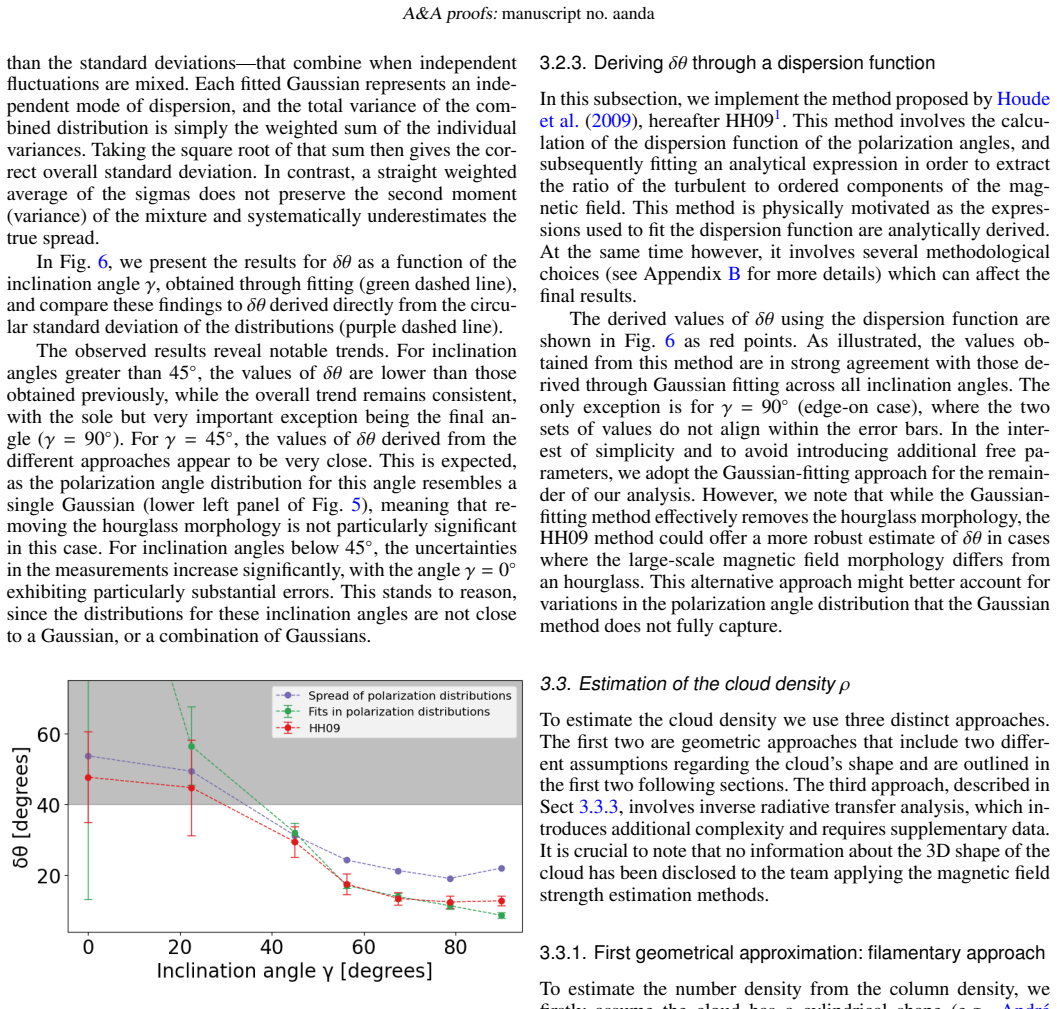
- [Section 3.2.3 footnote] The footnote states that the HH09 implementation was performed after the revision process and that the team already knew the true field strength values; the agreement between HH09 and the Gaussian-fit delta-theta in Fig. 6 should be interpreted with this potential bias in mind, and the main text should acknowledge this explicitly.
- [Section 3.3.3] The RADEX grid construction and the tolerance of 0.5 in the antenna temperature ratio are described qualitatively; please specify the exact grid spacing and the selection criterion so that the analysis is reproducible.
- [Eq. (12)] For a two-component Gaussian mixture, the total variance includes the between-component term A1*A2*(mu1 - mu2)^2; as written, Eq. (12) omits this term. Please clarify whether delta-theta is meant to represent the total spread of the polarization-angle distribution or only the turbulence-dominated component widths after removing the hourglass.
- [Section 5] The choice to compute chi-squared only for inclination angles gamma >= 45 degrees is not justified; since the paper also reports an accurate ST value at gamma = 22.5 degrees, please motivate or vary this cut.
- [Fig. 8] The labels for the parameter combinations (e.g., rho3, delta-v2, delta-theta2) are difficult to read at the displayed size; please annotate the best-performing panels directly or enlarge the figure.
- [Throughout] There are minor typographical issues, including 'obsrevations' in Section 2.2 and 'asses' in Section 1, and the double reference to 'Tritsis et al. 2025' with different A&A volume numbers should be checked.
Circularity Check
The central 'validation' of the three-step recipe is in-sample: the recipe is chosen by chi^2 against the true field of the same single simulation, and the claimed within-1sigma accuracy is then presented as a prediction.
-
fitted input called prediction
[Section 5 (Eq. 13, Fig. 10); recommendation repeated in Section 6 and Abstract]
"At this stage of our study, the actual magnetic field values from the simulation were disclosed ... In order to find which one of the 18 different combinations of parameters better estimates the actual magnetic field values, we calculate the chi^2 ... We observe that the models that behave better, for both methods, are those where the density is estimated using RADEX, dv from the second moment maps ... We decide to take as the best combination for both the methods, the one where every possible correction is applied."
The three-step recipe is not an independent prescription: it is the chi^2-best (for ST) among 18 combinations evaluated against the true B_POS of the same simulation after the truth was disclosed to the analysis team. The Abstract's claim that 'ST ... consistently remains within 1sigma from the true strength of the field' is therefore a report of the selected configuration's in-sample performance on the data used to select it, not an out-of-sample prediction. Appendix A, the only partially external check at a higher column-density threshold, explicitly fails to reproduce the monotonic cosine trend, so the central reliability claim rests on the same simulation that produced the selection.
full rationale
The ST and DCF formulas themselves are not circular: they are prior theoretical expressions (Skalidis & Tassis 2021; Davis 1951; Chandrasekhar & Fermi 1953), and the simulation's true magnetic field is an external ground truth, not an input to those formulas. The blind design also gives the intermediate estimates of rho, dv, and dtheta independent content, since those quantities were computed without knowing the true field. However, the paper's central deliverable is the specific three-step recipe (RADEX density, second-moment dv, Gaussian-fit dtheta) and the claim that this recipe 'reliably estimates' B_POS and remains within 1sigma. That deliverable is the output of a model-selection step: after the true field was disclosed, the authors computed chi^2 for all 18 parameter combinations and adopted the best (or, for DCF, a preferred) combination. The subsequent agreement is therefore partly fitted to the validation target rather than predicted from it. The only partially independent check, Appendix A with N_H2 >= 10^22 cm^-2, does not confirm the recipe; it shows the methods lose accuracy and no longer follow the expected monotonic trend. This in-sample selection constitutes a real but partial circularity: the physical comparison of ST versus DCF retains independent content, while the claimed reliability of the recommended recipe is not independently demonstrated. The DCF case also weakens the selection argument, since Fig. 10 shows the lowest chi^2 for DCF uses the circular standard deviation for dtheta, yet the paper adopts the Gaussian fit for both methods because it applies 'every possible correction'; thus the recipe is partly a prior choice, not purely a chi^2-forced optimum. No load-bearing self-citation chain is present: the ST method is tested against a new simulation rather than merely asserted by self-citation. Overall, the central accuracy claim is partially circular by construction of its validation, justifying a score of 6.
Assumptions & free parameters
free parameters (4)
- Column-density threshold (NH2 >= 1e21 cm^-2) =
1e21 cm^-2
- DCF correction factor f =
0.5
- RADEX grid bounds and CO abundance range =
n_H2 = 1e2-1e4 cm^-3; X_CO = 5e-7 to 7e-5
- Effective cloud depth Delta' for the HH09 dispersion function =
POS cloud dimension
assumptions (5)
- domain assumption Energy equipartition between turbulent kinetic energy and magnetic energy fluctuations (Eqs. 2 and 7)
- domain assumption Ideal MHD, flux freezing, and isothermal 10 K gas
- ad hoc to paper A single collapsing-cloud realization represents real self-gravitating clouds
- domain assumption 12CO traces the turbulence relevant for equipartition
- ad hoc to paper The CO-weighted median POS field is the appropriate ground truth
Cite this review
Pith. "Pith review of A three-step approach to reliably estimate magnetic field strengths in star-forming regions." pith.science (2026). https://pith.science/paper/ZVZPUM76
@misc{pith2026250706297,
  author       = {Pith},
  title        = {Pith review of: A three-step approach to reliably estimate magnetic field strengths in star-forming regions},
  year         = {2026},
  howpublished = {\url{https://pith.science/paper/ZVZPUM76}},
  note         = {Machine review of arXiv:2507.06297}
}
read the original abstract
The magnetic field is known to play a crucial role in star formation. Dust polarization is an effective tool for probing the morphology of the field, yet it does not directly trace its strength. Several methods have been developed, combining polarization and spectroscopic data, to estimate the strength of the magnetic field, including the DCF method, which relates these quantities to the magnetic-field strength under the assumption of Alfv\'enic turbulence. Skalidis & Tassis (2021) (ST), relaxed this assumption to account for the compressible modes, deriving more accurate estimates of the field strength. We evaluate the accuracy of these methods in star-forming regions and propose a systematic approach for calculating the key observational parameters involved: the velocity dispersion (dv), the dispersion of polarization angles (d\theta), and the cloud density (rho). We use a 3D MHD chemodynamical simulation of a turbulent molecular cloud and generate synthetic observations, for seven different inclination angles. We employ various approaches for estimating the parameters dv, d\theta, and rho and find that the approach used to calculate these parameters plays a crucial role in estimating the magnetic field strength. We show that the value probed by both the DCF and ST methods corresponds to the median of the molecular-species-weighted POS component of the magnetic field. The ST outperforms DCF, accurately following the expected cosine trend with respect to the inclination angle, and remains within 1\sigma from the true strength of the field. Based on our analysis, we proposed that, in self-gravitating clouds, the intrinsic parameters (rho, dv, d\theta) should be calculated as follows: rho using radiative transfer analysis, dv using the second moment maps, and d\theta by fitting Gaussians to the polarization angle distributions to remove the contribution of the hourglass morphology.
Figures


Figures from the paper (7 more)




Forward citations
Cited by 1 Pith paper
-
Challenges in probing turbulent and magnetic support in cores: the W43-MM1 protocluster case study
Simplified virial analyses of W43-MM1 cores overestimate non-thermal support because linewidths include organized motions of 1–3 km/s and surface terms are omitted, producing unexpectedly high stability fractions.
Reference graph
Works this paper leans on
-
[1]
, " * write output.state after.block = add.period write newline
ENTRY address archiveprefix author booktitle chapter edition editor howpublished institution eprint journal key month note number organization pages publisher school series title type volume year label extra.label sort.label short.list INTEGERS output.state before.all mid.sentence after.sentence after.block FUNCTION init.state.consts #0 'before.all := #1 ...
-
[2]
write newline
" write newline "" before.all 'output.state := FUNCTION n.dashify 't := "" t empty not t #1 #1 substring "-" = t #1 #2 substring "--" = not "--" * t #2 global.max substring 't := t #1 #1 substring "-" = "-" * t #2 global.max substring 't := while if t #1 #1 substring * t #2 global.max substring 't := if while FUNCTION word.in bbl.in " " * FUNCTION format....
-
[3]
Andersson, B.-G., Lazarian, A., & Vaillancourt, J. E.\ 2015, , 53, 501. doi:10.1146/annurev-astro-082214-122414
-
[4]
doi:10.1051/0004-6361/201014666
Andr \'e , P., Men'shchikov, A., Bontemps, S., et al.\ 2010, , 518, L102. doi:10.1051/0004-6361/201014666
-
[5]
doi:10.1051/0004-6361/201116596
Arzoumanian, D., Andr \'e , P., Didelon, P., et al.\ 2011, , 529, L6. doi:10.1051/0004-6361/201116596
-
[6]
S., Hasegawa, T., et al.\ 2021, , 647, A78
Arzoumanian, D., Furuya, R. S., Hasegawa, T., et al.\ 2021, , 647, A78. doi:10.1051/0004-6361/202038624
-
[7]
Beattie, J. R., Federrath, C., Klessen, R. S., et al.\ 2025, Nature Astronomy. doi:10.1038/s41550-025-02551-5
-
[8]
R., Federrath, C., & Seta, A.\ 2020, , 498, 2, 1593
Beattie, J. R., Federrath, C., & Seta, A.\ 2020, , 498, 2, 1593. doi:10.1093/mnras/staa2257
Show all 92 references
-
[9]
R., Krumholz, M
Beattie, J. R., Krumholz, M. R., Skalidis, R., et al.\ 2022, , 515, 4, 5267. doi:10.1093/mnras/stac2099
2022 doi
-
[10]
T., Padovani, M., Girart, J
Beltr \'a n, M. T., Padovani, M., Girart, J. M., et al.\ 2019, , 630, A54. doi:10.1051/0004-6361/201935701
2019 doi
-
[11]
C., et al.\ 2024, , 684, A212
Be s li \'c , I., Coud \'e , S., Lis, D. C., et al.\ 2024, , 684, A212. doi:10.1051/0004-6361/202348376
2024 doi
-
[12]
& Hameiri, E.\ 1988, Physics of Fluids, 31, 5, 1153
Bhattacharjee, A. & Hameiri, E.\ 1988, Physics of Fluids, 31, 5, 1153. doi:10.1063/1.866744
1988 doi
-
[13]
S., & Spangler, S
Bhattacharjee, A., Ng, C. S., & Spangler, S. R.\ 1998, , 494, 1, 409. doi:10.1086/305184
1998 doi
-
[14]
doi:10.1051/0004-6361/201937104
Bonne, L., Schneider, N., Bontemps, S., et al.\ 2020, , 641, A17. doi:10.1051/0004-6361/201937104
2020 doi
-
[15]
& Fermi, E.\ 1953, , 118, 113
Chandrasekhar, S. & Fermi, E.\ 1953, , 118, 113. doi:10.1086/145731
1953 doi
-
[16]
& Yoo, H.\ 2016, , 821, 1, 21
Cho, J. & Yoo, H.\ 2016, , 821, 1, 21. doi:10.3847/0004-637X/821/1/21
2016 doi
-
[17]
doi:10.3847/1538-4357/ad88ed
Choi, Y., Kwon, W., Pattle, K., et al.\ 2024, , 977, 1, 32. doi:10.3847/1538-4357/ad88ed
2024 doi
-
[18]
doi:10.3847/1538-4357/ab1b23
Coud \'e , S., Bastien, P., Houde, M., et al.\ 2019, , 877, 2, 88. doi:10.3847/1538-4357/ab1b23
2019 doi
-
[19]
M.\ 2012, , 50, 29
Crutcher, R. M.\ 2012, , 50, 29. doi:10.1146/annurev-astro-081811-125514
2012 doi
-
[20]
doi:10.1103/PhysRev.81.890.2
Davis, L.\ 1951, Physical Review, 81, 5, 890. doi:10.1103/PhysRev.81.890.2
1951 doi
-
[21]
B., & Fisher, R.\ 2008, Physica Scripta Volume T, 132, 014046
Dubey, A., Reid, L. B., & Fisher, R.\ 2008, Physica Scripta Volume T, 132, 014046. doi:10.1088/0031-8949/2008/T132/014046
2008 doi
-
[22]
S., et al.\ 2021, , 912, 2, L27
Eswaraiah, C., Li, D., Furuya, R. S., et al.\ 2021, , 912, 2, L27. doi:10.3847/2041-8213/abeb1c
2021 doi
-
[23]
doi:10.1086/587479
Falceta-Gon c alves, D., Lazarian, A., & Kowal, G.\ 2008, , 679, 1, 537. doi:10.1086/587479
2008 doi
-
[24]
doi:10.1017/S0022377816001069
Federrath, C.\ 2016, Journal of Plasma Physics, 82, 6, 535820601. doi:10.1017/S0022377816001069
2016 doi
-
[25]
S., et al.\ 2010, , 512, A81
Federrath, C., Roman-Duval, J., Klessen, R. S., et al.\ 2010, , 512, A81. doi:10.1051/0004-6361/200912437
2010 doi
-
[26]
S., et al.\ 2022, Astrophysics Source Code Library
Federrath, C., Roman-Duval, J., Klessen, R. S., et al.\ 2022, Astrophysics Source Code Library. ascl:2204.001
2022
-
[27]
M.\ 2011, , 535, A44
Frau, P., Galli, D., & Girart, J. M.\ 2011, , 535, A44. doi:10.1051/0004-6361/201117813
2011 doi
-
[28]
doi:10.1086/317361
Fryxell, B., Olson, K., Ricker, P., et al.\ 2000, , 131, 1, 273. doi:10.1086/317361
2000 doi
-
[29]
M., Rao, R., & Marrone, D
Girart, J. M., Rao, R., & Marrone, D. P.\ 2006, Science, 313, 5788, 812. doi:10.1126/science.1129093
2006 doi
-
[30]
M., Beltr \'a n, M
Girart, J. M., Beltr \'a n, M. T., Zhang, Q., et al.\ 2009, Science, 324, 5933, 1408. doi:10.1126/science.1171807
2009 doi
-
[31]
doi:10.1051/0004-6361/202142713
Gong, Y., Liu, S., Wang, J., et al.\ 2022, , 663, A82. doi:10.1051/0004-6361/202142713
2022 doi
-
[33]
R., Millman, K
Harris, C. R., Millman, K. J., van der Walt, S. J., et al.\ 2020, , 585, 7825, 357. doi:10.1038/s41586-020-2649-2
2020 doi
-
[34]
G., Mac Low, M.-M., et al.\ 2001, , 561, 2, 800
Heitsch, F., Zweibel, E. G., Mac Low, M.-M., et al.\ 2001, , 561, 2, 800. doi:10.1086/323489
2001 doi
-
[35]
& Inutsuka, S.-
Hennebelle, P. & Inutsuka, S.-. ichiro .\ 2019, Frontiers in Astronomy and Space Sciences, 6, 5. doi:10.3389/fspas.2019.00005
2019
-
[36]
H., Kirby, L., Dotson, J
Hildebrand, R. H., Kirby, L., Dotson, J. L., et al.\ 2009, , 696, 1, 567. doi:10.1088/0004-637X/696/1/567
2009 doi
-
[37]
E., Hildebrand, R
Houde, M., Vaillancourt, J. E., Hildebrand, R. H., et al.\ 2009, , 706, 2, 1504. doi:10.1088/0004-637X/706/2/1504
2009 doi
-
[38]
doi:10.1093/mnras/stac972
Hu, Y., Federrath, C., Xu, S., et al.\ 2022, , 513, 2, 2100. doi:10.1093/mnras/stac972
2022 doi
-
[39]
doi:10.1093/mnras/stad3766
Hu, Y., Lazarian, A., Wu, Y., et al.\ 2024, , 527, 4, 11240. doi:10.1093/mnras/stad3766
2024 doi
-
[40]
D.\ 2007, Computing in Science and Engineering, 9, 3, 90
Hunter, J. D.\ 2007, Computing in Science and Engineering, 9, 3, 90. doi:10.1109/MCSE.2007.55
2007 doi
-
[41]
doi:10.3847/1538-4357/ac99e0
Hwang, J., Kim, J., Pattle, K., et al.\ 2022, , 941, 1, 51. doi:10.3847/1538-4357/ac99e0
2022 doi
-
[42]
Kalberla, P. M. W. & Haud, U.\ 2023, , 673, A101. doi:10.1051/0004-6361/202245200
2023 doi
-
[43]
doi:10.3847/1538-4357/acd6f2
Karoly, J., Ward-Thompson, D., Pattle, K., et al.\ 2023, , 952, 1, 29. doi:10.3847/1538-4357/acd6f2
2023 doi
-
[44]
K., Chen, C.-Y., Fissel, L
King, P. K., Chen, C.-Y., Fissel, L. M., et al.\ 2019, , 490, 2, 2760. doi:10.1093/mnras/stz2628
2019 doi
-
[45]
& Basu, S.\ 2003, , 595, 2, 842
Kudoh, T. & Basu, S.\ 2003, , 595, 2, 842. doi:10.1086/377495
2003 doi
-
[46]
doi:10.3847/1538-4357/ac4bbe
Kwon, W., Pattle, K., Sadavoy, S., et al.\ 2022, , 926, 2, 163. doi:10.3847/1538-4357/ac4bbe
2022 doi
-
[47]
K., Pitrou, A., & Seibert, S.\ 2015, Proc
Lam, S. K., Pitrou, A., & Seibert, S.\ 2015, Proc. Second Workshop on the LLVM Compiler Infrastructure in HPC, 1. doi:10.1145/2833157.2833162
2015
-
[48]
W., Yuen, K
Lazarian, A., Ho, K. W., Yuen, K. H., et al.\ 2025, , 978, 1, 88. doi:10.3847/1538-4357/ad8d49
2025 doi
-
[49]
I., Fern \'a ndez-L \'o pez, M., Storm, S., et al.\ 2014, , 797, 2, 76
Lee, K. I., Fern \'a ndez-L \'o pez, M., Storm, S., et al.\ 2014, , 797, 2, 76. doi:10.1088/0004-637X/797/2/76
2014 doi
-
[50]
S., Lopez-Rodriguez, E., Ajeddig, H., et al.\ 2022, , 510, 4, 6085
Li, P. S., Lopez-Rodriguez, E., Ajeddig, H., et al.\ 2022, , 510, 4, 6085. doi:10.1093/mnras/stab3448
2022 doi
-
[51]
doi:10.3847/1538-4357/ab0958
Liu, J., Qiu, K., Berry, D., et al.\ 2019, , 877, 1, 43. doi:10.3847/1538-4357/ab0958
2019 doi
-
[52]
doi:10.3847/1538-4357/ac0cec
Liu, J., Zhang, Q., Commer c on, B., et al.\ 2021, , 919, 2, 79. doi:10.3847/1538-4357/ac0cec
2021 doi
-
[53]
& Goldreich, P.\ 2001, , 554, 2, 1175
Maron, J. & Goldreich, P.\ 2001, , 554, 2, 1175. doi:10.1086/321413
2001 doi
-
[54]
M.\ 2022, Frontiers in Astronomy and Space Sciences, 9, 949223
Maury, A., Hennebelle, P., & Girart, J. M.\ 2022, Frontiers in Astronomy and Space Sciences, 9, 949223. doi:10.3389/fspas.2022.949223
2022
-
[55]
Mouschovias, T. C. & Spitzer, L.\ 1976, , 210, 326. doi:10.1086/154835
1976 doi
-
[56]
Myers, P. C. & Goodman, A. A.\ 1991, , 373, 509. doi:10.1086/170070
1991 doi
-
[57]
C., Stone, J
Ostriker, E. C., Stone, J. M., & Gammie, C. F.\ 2001, , 546, 2, 980. doi:10.1086/318290
2001 doi
-
[58]
T., et al.\ 2001, , 559, 2, 1005
Padoan, P., Goodman, A., Draine, B. T., et al.\ 2001, , 559, 2, 1005. doi:10.1086/322504
2001 doi
-
[59]
doi:10.3847/0004-637X/822/1/11
Padoan, P., Pan, L., Haugb lle, T., et al.\ 2016, , 822, 1, 11. doi:10.3847/0004-637X/822/1/11
2016 doi
-
[60]
M., et al.\ 2021, , 912, 2, 159
Palau, A., Zhang, Q., Girart, J. M., et al.\ 2021, , 912, 2, 159. doi:10.3847/1538-4357/abee1e
2021 doi
-
[61]
V., Psaradaki, I., & Tassis, K.\ 2016, , 462, 2, 1517
Panopoulou, G. V., Psaradaki, I., & Tassis, K.\ 2016, , 462, 2, 1517. doi:10.1093/mnras/stw1678
2016 doi
- [62]
-
[63]
doi:10.3847/1538-4357/abcc6c
Pattle, K., Lai, S.-P., Di Francesco, J., et al.\ 2021, , 907, 2, 88. doi:10.3847/1538-4357/abcc6c
2021 doi
-
[64]
doi:10.3847/1538-4357/aa80e5
Pattle, K., Ward-Thompson, D., Berry, D., et al.\ 2017, , 846, 2, 122. doi:10.3847/1538-4357/aa80e5
2017 doi
-
[65]
M., et al.\ 2014, , 794, 1, L18
Qiu, K., Zhang, Q., Menten, K. M., et al.\ 2014, , 794, 1, L18. doi:10.1088/2041-8205/794/1/L18
2014 doi
-
[66]
doi:10.3847/2041-8213/ad660c
Saha, P., Sanhueza, P., Padovani, M., et al.\ 2024, , 972, 1, L6. doi:10.3847/2041-8213/ad660c
2024 doi
-
[67]
P., Busquet, G., Franco, G
Santos, F. P., Busquet, G., Franco, G. A. P., et al.\ 2016, , 832, 2, 186. doi:10.3847/0004-637X/832/2/186
2016 doi
-
[68]
W.\ 1979, On Optimal and Data-Based Histograms, Biometrika, 66(3), 605--610
Scott, D. W.\ 1979, On Optimal and Data-Based Histograms, Biometrika, 66(3), 605--610
1979
-
[69]
R., et al.\ 2008, , 687, 2, 1075
Sheffer, Y., Rogers, M., Federman, S. R., et al.\ 2008, , 687, 2, 1075. doi:10.1086/591484
2008 doi
- [70]
-
[71]
doi:10.1051/0004-6361/202345880
Skalidis, R., Gkimisi, K., Tassis, K., et al.\ 2023, , 673, A76. doi:10.1051/0004-6361/202345880
2023 doi
-
[72]
R., et al.\ 2021, , 656, A118
Skalidis, R., Sternberg, J., Beattie, J. R., et al.\ 2021, , 656, A118. doi:10.1051/0004-6361/202142045
2021 doi
-
[73]
& Tassis, K.\ 2021, , 647, A186
Skalidis, R. & Tassis, K.\ 2021, , 647, A186. doi:10.1051/0004-6361/202039779
2021 doi
-
[74]
V., et al.\ 2022, , 665, A77
Skalidis, R., Tassis, K., Panopoulou, G. V., et al.\ 2022, , 665, A77. doi:10.1051/0004-6361/202142512
2022 doi
-
[75]
doi:10.1051/0004-6361/202346072
Skalidis, R., Tassis, K., & Pavlidou, V.\ 2023, , 672, L3. doi:10.1051/0004-6361/202346072
2023 doi
-
[76]
D., Alves, F., Boulanger, F., et al.\ 2016, , 596, A93
Soler, J. D., Alves, F., Boulanger, F., et al.\ 2016, , 596, A93. doi:10.1051/0004-6361/201628996
2016 doi
-
[77]
W., Looney, L
Stephens, I. W., Looney, L. W., Kwon, W., et al.\ 2013, , 769, 1, L15. doi:10.1088/2041-8205/769/1/L15
2013 doi
-
[78]
& Federrath, C.\ 2022, , 509, 4, 5237
Stewart, M. & Federrath, C.\ 2022, , 509, 4, 5237. doi:10.1093/mnras/stab3313
2022 doi
-
[79]
doi:10.1051/epjconf/202226500022
Tafalla, M., Usero, A., & Hacar, \'A .\ 2022, European Physical Journal Web of Conferences, 265, 00022. doi:10.1051/epjconf/202226500022
2022
-
[80]
doi:10.1051/0004-6361/202452013
Tritsis, A., Basu, S., & Federrath, C.\ 2025, , 695, A18. doi:10.1051/0004-6361/202452013
2025 doi
-
[81]
doi:10.1051/0004-6361/202453265
Tritsis, A., Basu, S., & Federrath, C.\ 2025, , 696, A35. doi:10.1051/0004-6361/202453265
2025 doi
-
[82]
doi:10.1093/mnras/stab3740
Tritsis, A., Federrath, C., Willacy, K., et al.\ 2022, , 510, 3, 4420. doi:10.1093/mnras/stab3740
2022 doi
- [83]
-
[84]
V., Mouschovias, T
Tritsis, A., Panopoulou, G. V., Mouschovias, T. C., et al.\ 2015, , 451, 4, 4384. doi:10.1093/mnras/stv1133
2015 doi
-
[85]
doi:10.1093/mnras/sty1152
Tritsis, A., Yorke, H., & Tassis, K.\ 2018, , 478, 2, 2056. doi:10.1093/mnras/sty1152
2018 doi
- [86]
-
[87]
J., Smith, B
Turk, M. J., Smith, B. D., Oishi, J. S., et al.\ 2011, , 192, 1, 9. doi:10.1088/0067-0049/192/1/9
2011 doi
-
[88]
doi:10.1051/0004-6361/202243633
Valdivia, V., Maury, A., & Hennebelle, P.\ 2022, , 668, A83. doi:10.1051/0004-6361/202243633
2022 doi
-
[89]
van der Tak, F. F. S., Black, J. H., Sch \"o ier, F. L., et al.\ 2007, , 468, 2, 627. doi:10.1051/0004-6361:20066820
2007 doi
-
[90]
E., et al.\ 2020, Nature Methods, 17, 261
Virtanen, P., Gommers, R., Oliphant, T. E., et al.\ 2020, Nature Methods, 17, 261. doi:10.1038/s41592-019-0686-2
2020 doi
-
[91]
doi:10.3847/1538-4357/acbea4
Ward-Thompson, D., Karoly, J., Pattle, K., et al.\ 2023, , 946, 2, 62. doi:10.3847/1538-4357/acbea4
2023 doi
-
[92]
doi:10.3847/1538-4357/ada8a0
Xu, D., Karcheski, J., Law, C.-Y., et al.\ 2025, , 980, 1, 52. doi:10.3847/1538-4357/ada8a0
2025 doi
- [93]
Reviewed August 6, 2026 · model on record in the stance chip above.
Discussion (0). Continue with ORCID to comment.