REVIEW 4 major objections 6 minor 80 references
Exploring substructures in the Milky Way halo Neural networks applied to Gaia and APOGEE DR 17
T0 review · 4 major / 6 minor · reviewed 2026-08-06 · deepseek-v4-flash
Pith's one-line read A pipeline that feeds chemistry and stellar orbits through three neural networks recovers 80% of globular clusters in the APOGEE halo sample and identifies a new stream candidate, Arnus I.
desk verdict CREEK is a credible new chemo-dynamical tagging pipeline with an honest benchmark, but the GES split and Arnus I claims rest on reachability dips without a null-hypothesis baseline and need more work. read the letter →
The pith
A machine-rendered reading of the paper's core claim, the machinery that carries it, and where it could break.
The reading
What carries the argument
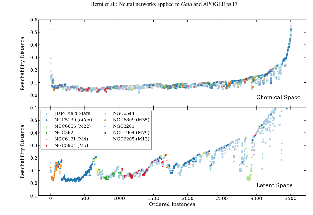
The load-bearing object is the graph built by the Siamese network and smoothed by the GNN autoencoder. A Siamese neural network is a twin-branch net that takes pairs of stars and outputs the probability they share the same orbit; here it is trained on orbital actions of globular-cluster members. Pairs above a 0.8 threshold become edges in a graph whose nodes carry chemical abundances. A graph-neural-network autoencoder then aggregates each node's chemistry with that of its linked neighbours, compresses the result to a five-dimensional latent space, and reconstructs the inputs; OPTICS, a density-clustering algorithm, finds valleys in the reachability plot that correspond to chemo-dynamically coherent groups. The key step is that chemistry is propagated only between stars the Siamese network judges dynamically similar, so clusters and streams become denser in latent space than they are in raw abundance space.
What would settle it
Re-run CREEK on the same APOGEE sample after replacing the orbital actions of field stars with scrambled values while preserving the cluster actions; if the known streams and the two Gaia-Enceladus dips still appear, the dynamical link is not doing the work. A more direct test is to apply CREEK to synthetic halo simulations with injected, artificially disrupted streams of known dynamical age and measure how the recovery fraction falls as the debris phase-mixes.
Extended reading notes
Core claim
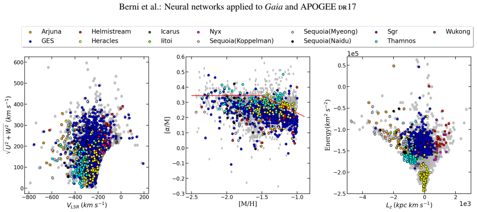
The central claim is that chemical abundances and orbital invariants can be integrated through neural networks into a single clustering framework that detects both intact and disrupted halo structures. CREEK first computes standardised orbital actions ($J_R$, $J_\phi$, $J_Z$) for each star, trains a Siamese network with equal numbers of same-cluster and different-cluster pairs drawn from the globular clusters, and links stars whose pairwise similarity exceeds 0.8. The resulting graph is fed to a graph autoencoder whose latent space carries chemistry smoothed along dynamical links; OPTICS then finds dense groups in that latent space. On the APOGEE halo sample this recovers eight of ten clusters above the 30% homogeneity/completeness threshold, places known streams in distinct dips of the reachability plot, splits Gaia-Enceladus into two populations that differ in energy and in several abundances, and yields Arnus I, a group of retrograde stars with in-situ-like chemistry.
Load-bearing premise
The load-bearing premise is that a neural network trained only on stars still bound in globular clusters learns a notion of 'same orbit' that also applies to stars that have been ripped out of their parent structure and mixed into the field.
Editorial extensions
If this is right
- Dynamics alone is insufficient for ancient, phase-mixed mergers; the paper demonstrates that adding chemistry through graph propagation recovers structures that are dispersed in velocity space.
- The Gaia-Enceladus selection of Horta et al. can be extended automatically: CREEK finds stars with consistent chemistry and dynamics outside the literature membership, and separates the stream into two energy and abundance subgroups.
- The method is repeatable and objective, applying the same thresholding to clusters, streams, and field stars, so future surveys can run it without manual stream selection.
- The Arnus I group is a testable prediction: if confirmed, it adds a new retrograde, in-situ-like accreted structure to the halo inventory.
- Running on 3548 stars takes about ten minutes on a CPU-only laptop, so the pipeline is positioned to scale to upcoming surveys such as 4MOST and WST.
Reading between the lines
- Extension: The decisive assumption is that dynamical similarity learned on intact globular clusters transfers to tidally heated and phase-mixed debris; a simulation-based test that injects streams with controlled dynamical ages could measure how recovery degrades with disruption.
- Extension: Because the Siamese-network threshold controls graph connectivity, the two Gaia-Enceladus dips and Arnus I should be re-tested with thresholds other than 0.8; stable groups would strengthen the claim, threshold-dependent ones would reveal where the method's sensitivity ends.
- Extension: The chemical input is limited to [M/H] and [alpha/M] by data quality; with higher-precision abundances, the same architecture might separate structures that overlap in alpha and metallicity.
- Extension: If Arnus I shares stars with Sequoia under a different membership selection, it may be a fragment of a larger progenitor rather than an independent stream; cross-survey comparison with GALAH could test that.
Editorial analysis
A structured set of objections, weighed in public.
Referee Report
Summary. The manuscript presents CREEK, an integrated machine-learning pipeline that combines a Siamese neural network (SNN) trained on orbital actions, a graph-neural-network autoencoder that propagates chemical abundances along action-similarity edges, and the OPTICS clustering algorithm. The method is applied to a sample of 3548 halo stars drawn from APOGEE DR17 and Gaia DR3. The authors report that CREEK recovers 8 of 10 globular clusters with completeness and homogeneity at least 30%, re-identifies known streams including Gaia-Enceladus-Sausage (GES) and Heracles, splits GES into two chemo-dynamically distinct substructures, and identifies a new candidate stream, Arnus I. The stated aim is to provide an objective, repeatable, data-driven method for chemical-dynamical tagging of stellar structures in current and future surveys.
Significance. If validated, CREEK would be a useful methodological contribution to Galactic archaeology, particularly for upcoming large spectroscopic surveys. The pipeline is clearly described, the use of external globular-cluster memberships and literature stream memberships is a genuine strength, and the comparison with the earlier chemical-tagging attempt of Chen et al. (2018) helps frame the improvement. The architecture is sensible, and the idea of combining conserved actions with chemical tagging through a graph autoencoder is worth pursuing. However, the significance of the specific discovery claims — the GES split and Arnus I — is currently limited by the absence of any null-hypothesis baseline, and the 80% globular-cluster recovery rate is weakened by the fact that the same clusters were used both to select the chemical tracers and to train the SNN. The paper is therefore a promising methods proof-of-concept whose headline astrophysical claims need substantially stronger validation.
major comments (4)
- [4.1.2 and 3.2] The central new discovery claims — the split of GES into two substructures and the identification of Arnus I — lack any null-hypothesis baseline. These structures are identified as dips in the OPTICS reachability plot obtained after the GNN autoencoder propagates chemical abundances along graph edges set by the SNN action-similarity threshold of 0.8. Under this construction, any overdense region in action space will be smoothed into a chemically coherent latent-space clump, so a reachability dip is expected even in the absence of a common progenitor. A permutation test (for example, shuffling abundances independently of actions, or applying the same pipeline to a smooth halo mock with identical selection function) is required before the dips can be interpreted as physical substructures. Without such a baseline, the GES split and Arnus I are not statistically supported.
- [2.3, 3.1, and 4.1.1] The 80% globular-cluster recovery rate is partly a training-set memory check rather than an independent validation. The element-selection metric in Section 2.3 and the SNN in Section 3.1 are both trained or tuned on the same globular clusters whose recovery is later reported in Section 4.1.1. This circularity should be addressed by a cross-validation design, for example training on a subset of clusters and testing recovery on held-out clusters, or by reporting recovery after excluding the clusters used for element selection and SNN training. In addition, the paper asserts in Section 3.1 that the SNN, although trained only on globular clusters, transfers to streams and field stars; this claim should be tested directly using literature stream memberships, since the transfer to disrupted, phase-mixed debris is the load-bearing assumption for all stream-related results.
- [4.1.2, GES analysis] The statistical test used to support the GES split is post hoc and non-decisive. The two samples are defined from the same dip structure that is being tested, ten elements are examined without any multiple-testing correction, and the authors themselves note that the abundance differences are within 1σ and that uncertainties 'prevent us from confirming their true existence.' The two-sample KS test should be supplemented with sample sizes, p-values for all elements, and effect sizes, and ideally with a test on an independently defined GES selection from the literature rather than on the dips that CREEK itself produced.
- [4.1.2, Arnus I] The Arnus I candidate is presented without any quantitative comparison to field contamination or to the null expectation. The overlap with a few Sequoia members is asserted visually, and the group's chemical and dynamical properties are described qualitatively. To support the claim of a new stream, the authors should provide a member list, quantify the overdensity relative to a smooth halo model or permutation baseline, and show that the group is not simply a chance clustering produced by the GNN smoothing. As it stands, the candidate status is preliminary and should be framed as such in the abstract and conclusions.
minor comments (6)
- [2.3, Eq. (1)] Equation (1) is unclear as printed: the summation notation 'i,jX' and the placement of Nstars in the numerator/denominator need to be defined rigorously, since this metric is central to the element-selection step.
- [3.1] The SNN link threshold of 0.8 is a free parameter that strongly affects the graph structure and therefore all downstream results. The paper should justify this choice quantitatively, for example with a precision-recall curve on the validation pairs, and show the sensitivity of the recovered clusters and streams to this threshold.
- [4.1.1] The recovery denominator should be stated explicitly: Table 1 lists ten clusters with more than ten members, and eight are recovered, giving the 80% figure. The text should also clarify whether 'recovered' is assessed against all ten clusters or only against those that appear as distinct OPTICS groups.
- [Figures 6, 7, and 8] The x-axis of the reachability plots is labelled 'ordered instances,' which is not explained in any figure caption. The authors should describe how OPTICS ordering works and, importantly, how the boundaries of the dips assigned to GES, Heracles, and Arnus I were chosen, since the definition of a 'dip' is not an automated step.
- [4.1.2 and 5] The number of stars in each GES dip and in Arnus I is not reported, making it difficult to evaluate the significance of the KS tests and the credibility of the Arnus I overdensity. Please add these numbers to the text or Table.
- [Throughout] The name of the method appears inconsistently as 'Creek' and 'CREEK'; please use one spelling consistently. Also, the paper has no code availability statement; for a methods-focused paper, releasing the code and the exact trained configurations would substantially strengthen reproducibility.
Circularity Check
GC recovery benchmark is partly in-sample and the GES split re-tests abundances used to build the latent space; stream re-identification retains independent grounding.
-
fitted input called prediction
[Sec. 2.3 (Eq. 1 element-selection metric); Sec. 3.1 (SNN training pairs); Sec. 4.1.1 (GC recovery benchmark)]
"In order to choose the best elements, we based our selection on the abundances of globular clusters, selecting the best elements to identify globular clusters from field halo stars. ... We applied C reek algorithm to the APOGEE dataset to test its ability to recover globular clusters."
The chemical input features ([M/H], [α/M]) were selected by maximizing inter-cluster vs. intra-cluster separation among the globular clusters themselves (Eq. 1), and the SNN's dynamical-similarity model was trained on same-cluster/different-cluster pairs drawn from those same clusters ('We selected 2250 pairs of stars from the same cluster and an equal number of pairs from different clusters'). The reported 80% GC recovery is then measured on the same clusters that supplied the training labels and feature-selection metric. This is an in-sample fit/memory benchmark, not an out-of-sample prediction; the unsupervised autoencoder and OPTICS steps make the recovery non-trivial but do not remove the circularity of using the target set to build the learnable components.
-
self definitional
[Sec. 4.1.2, GES subsection and Fig. 9; Sec. 3.2 (GNN latent-space input)]
"We then examined the abundances of other elements to determine whether they reveal two distinct chemical structures. ... We find that α-elements and Al are fairly consistently separated, with the first dip showing higher abundances than the second. ... This likely reflects the fact that C reek used α-elements and [M/H] to distinguish the O ptics groups."
The two GES sub-groups are defined as two dips in the OPTICS reachability plot of the latent space produced by the GNN autoencoder, whose only chemical inputs are [M/H] and [α/M] and whose edges are the SNN action-similarity links. KS-testing [M/H], [Mg/Fe], [Si/Fe], and [O/Fe] for the two dips largely re-tests the same chemical features used to construct the separation, so a difference is expected by construction rather than independently discovered. The paper itself concedes the differences are within 1σ and that uncertainties 'prevent us from confirming their true existence.' The Ce/Ni abundances provide some independent signal, but the headline claim of two chemo-dynamically distinct GES substructures is partly self-definitional.
full rationale
The pipeline is not wholly circular: the GNN autoencoder and OPTICS run unsupervised on field stars, and the re-identification of known streams is checked against external Horta et al. (2023) memberships. Self-citations (Giribaldi & Smiljanic 2023; Schiappacasse-Ulloa et al. 2025) are not load-bearing for the method's validity. The partial circularity is concentrated in two validation steps: (1) the globular-cluster recovery benchmark is evaluated on the same clusters used to select the chemical tracers and to train the SNN, so the 80% figure is partly a training-set memory check; and (2) the GES sub-structure split is read from dips in a latent space built on [M/H] and [α/M] and then 'confirmed' by KS tests on those same abundances. The Arnus I candidate is not circular by the same logic; its weakness is the absence of a null-hypothesis/permutation baseline, which is a correctness risk rather than a definitional reduction.
Assumptions & free parameters
free parameters (6)
- SNN link probability threshold =
0.8
- OPTICS xi =
0.001
- OPTICS min_samples =
7
- Autoencoder latent dimension =
5
- Globular cluster recovery thresholds =
H>=0.3, C>=0.3
- Chemical input features =
[M/H] and [alpha/M]
assumptions (5)
- domain assumption Actions (JR, Jphi, JZ) are conserved integrals of motion for stars in a static axisymmetric potential, at least to first approximation.
- domain assumption Photospheric chemical abundances are invariant over time and are shared by stars from a common progenitor.
- ad hoc to paper Dynamical similarity learned from globular clusters transfers to field halo stars and streams.
- domain assumption External membership catalogs used as ground truth (Vasiliev and Baumgardt 2021 for clusters, Horta et al. 2023 for streams) are complete and correct.
- domain assumption Orbits computed with AGAMA in the McMillan potential are accurate enough for the actions.
invented entities (2)
-
Arnus I (candidate stream)
-
Gaia Enceladus substructure split (two dips)
Cite this review
Pith. "Pith review of Exploring substructures in the Milky Way halo Neural networks applied to Gaia and APOGEE DR 17." pith.science (2026). https://pith.science/paper/4MQEYSEU
@misc{pith2026250708074,
  author       = {Pith},
  title        = {Pith review of: Exploring substructures in the Milky Way halo Neural networks applied to Gaia and APOGEE DR 17},
  year         = {2026},
  howpublished = {\url{https://pith.science/paper/4MQEYSEU}},
  note         = {Machine review of arXiv:2507.08074}
}
read the original abstract
The identification of stellar structures in the Galactic halo, including stellar streams and merger remnants, often relies on the dynamics of their constituent stars. However, this approach has limitations due to the complex dynamical interactions between these structures and their environment. Perturbations such as tidal forces exerted by the Milky Way, the potential escape of stars, and passages through the Galactic plane can result in the loss of dynamical coherence of stars in these structures. Consequently, relying solely on dynamics may be insufficient for detecting such disrupted or dispersed remnants. We combine chemistry and dynamics, integrated through a system of neural networks, to develop a clustering method for identifying accreted structures in the Galactic halo. We developed an integrated approach combining Siamese neural networks (SNNs), graph neural networks (GNNs), autoencoders, and the OPTICS algorithm to create a comprehensive procedure named CREEK. This method is designed to uncover stellar structures in the Galactic halo. Initially, CREEK was trained on known globular clusters (GCs) and then applied to the dataset to identify stellar streams. CREEK successfully recovered 80% of the GCs present in the APOGEE dataset, re-identified several known stellar streams, and identified a potential new stream. Additionally, within highly populated stellar structures, CREEK can identify substructures that exhibit distinct chemical compositions and orbital energies. This approach provides an objective data-driven method for selecting stars associated with streams and stellar structures in general.
Figures


Figures from the paper (5 more)



Reference graph
Works this paper leans on
-
[1]
2025, arXiv preprint arXiv:2502.20436
Aguado-Agelet, F., Massari, D., Monelli, M., et al. 2025, arXiv preprint arXiv:2502.20436
arXiv 2025
- [2]
-
[3]
2016, arXiv e-prints, arXiv:1611.01491
Arora, R., Basu, A., Mianjy, P., & Mukherjee, A. 2016, arXiv e-prints, arXiv:1611.01491
arXiv 2016
-
[4]
Bailer-Jones, C., Rybizki, J., Fouesneau, M., Demleitner, M., & Andrae, R. 2021, AJ, 161, 147
work page 2021
-
[5]
Beasley, M. A. 2020, Reviews in Frontiers of Modern Astrophysics: From Space Debris to Cosmology, 245
work page 2020
- [6]
-
[7]
Belokurov, V ., Erkal, D., Evans, N., Koposov, S., & Deason, A. J. 2018, MNRAS, 478, 611
work page 2018
- [8]
Show all 80 references
-
[9]
B., Evans, N
Belokurov, V ., Zucker, D. B., Evans, N. W., et al. 2006, ApJ, 642, L137
2006
-
[10]
2003, A&A, 410, 527
Bensby, T., Feltzing, S., & Lundström, I. 2003, A&A, 410, 527
2003
-
[11]
2015, A&A, 577, A47
Blanco-Cuaresma, S., Soubiran, C., Heiter, U., et al. 2015, A&A, 577, A47
2015
-
[12]
P., Conroy, C., et al
Bonaca, A., Naidu, R. P., Conroy, C., et al. 2021, ApJ, 909, L26
2021
-
[13]
& Price-Whelan, A
Bonaca, A. & Price-Whelan, A. M. 2025, New A Rev., 100, 101713
2025
-
[14]
W., Martell, S
Borsato, N. W., Martell, S. L., & Simpson, J. D. 2020, MNRAS, 492, 1370
2020
-
[15]
Bullock, J. S. & Johnston, K. V . 2005, ApJ, 635, 931
2005
-
[16]
& Lia, C
Carraro, G. & Lia, C. 2000, A&A, 357, 977
2000
-
[17]
G., et al
Carretta, E., Bragaglia, A., Gratton, R. G., et al. 2010, A&A, 516, A55
2010
-
[18]
2022, MNRAS, 513, 1557
Carrillo, A., Hawkins, K., Jofré, P., et al. 2022, MNRAS, 513, 1557
2022
-
[19]
2025, arXiv preprint arXiv:2503.02939
Ceccarelli, E., Massari, D., Aguado-Agelet, F., et al. 2025, arXiv preprint arXiv:2503.02939
2025 arXiv
-
[20]
A., et al
Chen, B., D’Onghia, E., Pardy, S. A., et al. 2018, ApJ, 860, 70
2018
-
[21]
& Gnedin, O
Chen, Y . & Gnedin, O. Y . 2024, OJA, 7, 23
2024
-
[22]
2021, Siamese Neural Networks: An Overview (New York, NY: Springer US), 73–94
Chicco, D. 2021, Siamese Neural Networks: An Overview (New York, NY: Springer US), 73–94
2021
-
[23]
P., Zaritsky, D., et al
Conroy, C., Naidu, R. P., Zaritsky, D., et al. 2019, ApJ, 887, 237
2019
-
[24]
P., Cole, S., Frenk, C., et al
Cooper, A. P., Cole, S., Frenk, C., et al. 2010, MNRAS, 406, 744 da Silva, A. R. & Smiljanic, R. 2023, A&A, 677, A74
2010
-
[25]
E., & Madau, P
Dai, B., Robertson, B. E., & Madau, P. 2018, ApJ, 858, 73
2018
-
[26]
2020, MNRAS, 493, 5195 de Graaff, A., Rix, H.-W., Carniani, S., et al
Das, P., Hawkins, K., & Jofré, P. 2020, MNRAS, 493, 5195 de Graaff, A., Rix, H.-W., Carniani, S., et al. 2024, A&A, 684, A87 de Jong, R. S., Agertz, O., Berbel, A. A., et al. 2019a, The Messenger, 175, 3 de Jong, R. S., Agertz, O., et al. 2019b, The Messenger, 175, 3 De Silva,...
2020
-
[27]
M., Helmi, A., et al
Dodd, E., Callingham, T. M., Helmi, A., et al. 2023, A&A, 670, L2 D’Onghia, E., Springel, V ., Hernquist, L., & Keres, D. 2010, ApJ, 709, 1138
2023
-
[28]
K., Feltzing, S., Sahlholdt, C
Feuillet, D. K., Feltzing, S., Sahlholdt, C. L., & Casagrande, L. 2020, MNRAS, 497, 109
2020
-
[29]
& Bland-Hawthorn, J
Freeman, K. & Bland-Hawthorn, J. 2002, ARA&A, 40, 487
2002
-
[30]
Gibbons, S. L. J., Belokurov, V ., & Evans, N. W. 2017, MNRAS, 464, 794
2017
-
[31]
2022, A&A, 666, A120
Gilmore, G., Randich, S., Worley, C., et al. 2022, A&A, 666, A120
2022
-
[32]
Giribaldi, R. E. & Smiljanic, R. 2023, A&A, 673, A18
2023
-
[33]
2005, in Proceedings
Gori, M., Monfardini, G., & Scarselli, F. 2005, in Proceedings. 2005 IEEE Inter- national Joint Conference on Neural Networks, 2005., V ol. 2, 729–734 vol. 2
2005
-
[34]
G., Carretta, E., & Bragaglia, A
Gratton, R. G., Carretta, E., & Bragaglia, A. 2012, A&A Rev., 20, 50
2012
-
[35]
J., Hogg, D
Griffith, E. J., Hogg, D. W., Hasselquist, S., et al. 2025, AJ, 169, 280
2025
-
[36]
2015, MNRAS, 453, 758
Hawkins, K., Jofre, P., Masseron, T., & Gilmore, G. 2015, MNRAS, 453, 758
2015
-
[37]
R., Majewski, S
Hayes, C. R., Majewski, S. R., Shetrone, M., et al. 2018, ApJ, 852, 49
2018
-
[38]
H., et al
Helmi, A., Babusiaux, C., Koppelman, H. H., et al. 2018, Nature, 563, 85
2018
-
[39]
& Tim de Zeeuw, P
Helmi, A. & Tim de Zeeuw, P. 2000, MNRAS, 319, 657
2000
-
[40]
A., Tian, H., & Sales, L
Helmi, A., Veljanoski, J., Breddels, M. A., Tian, H., & Sales, L. V . 2017, A&A, 598, A58
2017
-
[41]
P., Mackereth, J
Horta, D., Schiavon, R. P., Mackereth, J. T., et al. 2023, MNRAS, 520, 5671
2023
-
[42]
C., Dalton, G
Jin, S., Trager, S. C., Dalton, G. B., et al. 2023, MNRAS
2023
-
[43]
Johnson, C. I. & Pilachowski, C. A. 2010, ApJ, 722, 1373
2010
-
[44]
& Grebel, E
Jordi, K. & Grebel, E. K. 2010, A&A, 522, A71
2010
-
[45]
1933, Giorn Dell’inst Ital Degli Att, 4, 89
Kolmogorov, A. 1933, Giorn Dell’inst Ital Degli Att, 4, 89
1933
-
[46]
H., Bos, R
Koppelman, H. H., Bos, R. O., & Helmi, A. 2020, A&A, 642, L18
2020
-
[47]
C., et al
Lagarde, N., Reylé, C., Robin, A. C., et al. 2019, A&A, 621, A24
2019
-
[48]
M., Bovy, J., & Mackereth, J
Lane, J. M., Bovy, J., & Mackereth, J. T. 2022, MNRAS, 510, 5119
2022
-
[49]
M., Bovy, J., & Mackereth, J
Lane, J. M., Bovy, J., & Mackereth, J. T. 2023, MNRAS, 526, 1209 Lövdal, S. S., Ruiz-Lara, T., Koppelman, H. H., et al. 2022, A&A, 665, A57
2023
-
[50]
Mainieri, V . et al. 2024, arXiv e-prints, arXiv:2403.05398
2024 arXiv
-
[51]
R., Schiavon, R
Majewski, S. R., Schiavon, R. P., Frinchaboy, P. M., et al. 2017, AJ, 154, 94
2017
-
[52]
A., Sharma, S., et al
Malhan, K., Ibata, R. A., Sharma, S., et al. 2022, ApJ, 926, 107
2022
-
[53]
Martell, S. L. & Grebel, E. K. 2010, A&A, 519, A14
2010
-
[54]
L., Shetrone, M
Martell, S. L., Shetrone, M. D., Lucatello, S., et al. 2016, ApJ, 825, 146
2016
-
[55]
F., Venn, K
Martin, N. F., Venn, K. A., Aguado, D. S., et al. 2022, Nature, 601, 45
2022
-
[56]
2023, A&A, 680, A20
Massari, D., Aguado-Agelet, F., Monelli, M., et al. 2023, A&A, 680, A20
2023
-
[57]
H., & Helmi, A
Massari, D., Koppelman, H. H., & Helmi, A. 2019, A&A, 630, L4
2019
-
[58]
McMillan, P. J. 2016, MNRAS, stw2759
2016
-
[59]
W., De Silva, G., Sharma, S., & Zucker, D
Mitschang, A. W., De Silva, G., Sharma, S., & Zucker, D. B. 2013, MNRAS, 428, 2321
2013
-
[60]
L., et al
Monty, S., Belokurov, V ., Sanders, J. L., et al. 2024, MNRAS, 533, 2420
2024
-
[61]
2024, A&A, 690, A136
Mori, A., Di Matteo, P., Salvadori, S., et al. 2024, A&A, 690, A136
2024
-
[62]
2019, MNRAS, 487, 2718
Morinaga, Y ., Ishiyama, T., Kirihara, T., & Kinjo, K. 2019, MNRAS, 487, 2718
2019
-
[63]
Nissen, P. E. & Schuster, W. J. 2010, A&A, 511, L10
2010
-
[64]
2017, A&A, 601, A112 Pérez, A
Pancino, E., Romano, D., Tang, B., et al. 2017, A&A, 601, A112 Pérez, A. E. G., Prieto, C. A., Holtzman, J. A., et al. 2016, AJ, 151, 144
2017
-
[65]
2022, A&A, 666, A121
Randich, S., Gilmore, G., Magrini, L., et al. 2022, A&A, 666, A121
2022
-
[66]
2018, A&A, 620, A194
Recio-Blanco, A. 2018, A&A, 620, A194
2018
-
[67]
2017, MNRAS, 465, 1157
Rodrigues, M., Hammer, F., Flores, H., Puech, M., & Athanassoula, E. 2017, MNRAS, 465, 1157
2017
-
[68]
S., et al
Ruiz-Lara, T., Matsuno, T., Lövdal, S. S., et al. 2022, A&A, 665, A58
2022
-
[69]
2025, A&A, arXiv:2505.08399, in press
Schiappacasse-Ulloa, J., Magrini, L., Lucatello, S., et al. 2025, A&A, arXiv:2505.08399, in press
2025 arXiv
-
[70]
& Zinn, R
Searle, L. & Zinn, R. 1978, ApJ, 225, 357
1978
-
[71]
R., & Necib, L
Shih, D., Buckley, M. R., & Necib, L. 2024, MNRAS, stae446
2024
-
[72]
G., et al
Spina, L., Magrini, L., Sacco, G. G., et al. 2022, A&A, 668, A16 The MSE Science Team, Babusiaux, C., Bergemann, M., et al. 2019, arXiv e- prints, arXiv:1904.04907
2022 arXiv
-
[73]
B., Beers, T
Tissera, P. B., Beers, T. C., Carollo, D., & Scannapieco, C. 2014, MNRAS, 439, 3128
2014
-
[74]
2009, ARA&A, 47, 371
Tolstoy, E., Hill, V ., & Tosi, M. 2009, ARA&A, 47, 371
2009
-
[75]
& Shigeyama, T
Tsujimoto, T. & Shigeyama, T. 2003, ApJ, 590, 803
2003
-
[76]
2019, MNRAS, 482, 1525
Vasiliev, E. 2019, MNRAS, 482, 1525
2019
-
[77]
& Baumgardt, H
Vasiliev, E. & Baumgardt, H. 2021, MNRAS, 505, 5978
2021
-
[78]
G., & Cassisi, S
Villanova, S., Geisler, D., Gratton, R. G., & Cassisi, S. 2014, ApJ, 791, 107
2014
-
[79]
2019, MNRAS, 487, L47
Vincenzo, F., Spitoni, E., Calura, F., et al. 2019, MNRAS, 487, L47
2019
-
[80]
2022, The Innovation, 3 Article number, page 12 of 12
Yan, H., Li, H., Wang, S., et al. 2022, The Innovation, 3 Article number, page 12 of 12
2022
Reviewed August 6, 2026 · model on record in the stance chip above.
Discussion (0). Continue with ORCID to comment.