REVIEW 3 major objections 6 minor 54 references
OffsetCrust: Variable-Radius Offset Approximation with Power Diagrams
T0 review · 3 major / 6 minor · reviewed 2026-08-06 · deepseek-v4-flash
Pith's one-line read The variable-radius offset of a surface can be computed as the separator between two kinds of weighted sites in a power diagram, with displaced points placed along a radius-dependent direction.
desk verdict A practical variable-radius offset method with a clean core idea and strong experiments; Theorem 1 needs a real proof and the manifoldness claim is too strong, but it deserves serious peer review. read the letter →
The pith
A machine-rendered reading of the paper's core claim, the machinery that carries it, and where it could break.
The reading
What carries the argument
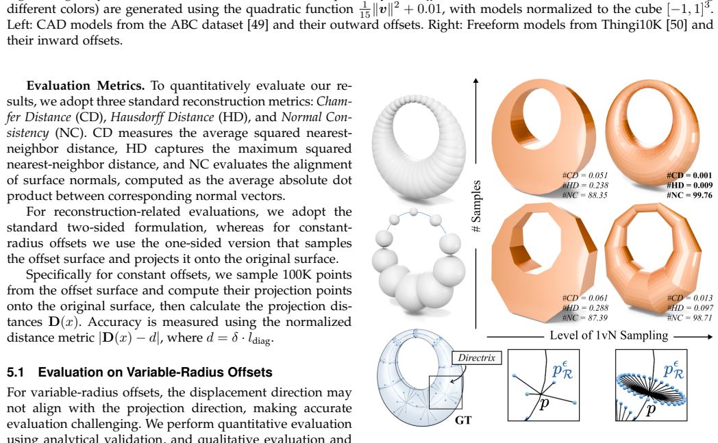
The central object is the power diagram of two weighted point sets: base samples $p$ with weight $R(p)^2$ and displaced samples $p^{\epsilon}_R=p+\epsilon\,n^{\mathrm{off}}_R(p)$ with weight $(R(p)-\epsilon)^2$. The offset surface is extracted as the separator between the two classes of power cells, and the load-bearing identity is equation (4): a point on the offset satisfies equal power distances to the two members of a matched pair exactly when it satisfies the generalized offset equation. Theorem 1 supplies the displacement direction that makes this identity track the true envelope, while the regularized least-squares step (equations (14)--(15)) fits each power-diagram vertex to the tangent-plane constraints $(v-p_i)\cdot n^{\mathrm{off}}_i=R(p_i)$ and thereby suppresses the misaligned facets that generic crust sampling produces.
What would settle it
Take a surface with an analytically known variable-radius offset, such as a sphere with $R(x)=1+a x$, compute the true contact direction $n^{\mathrm{off}}_R$ at several points from the envelope, and compare it with the rotated normal given by Theorem 1; a discrepancy beyond sampling and $\epsilon$ discretization error, or a failure of the power-diagram facet boundary to converge to $\phi(x)=0$ as samples increase, would refute the central claim.
Extended reading notes
Core claim
The central discovery is that the generalized distance function $\phi(x)=\min_{p\in S}(\|x-p\|-R(p))$ can be represented by a power diagram whose sites come in matched pairs. For any base point $p$ that contributes to the offset, the identity $\|p^{\mathrm{off}}_R-p\|^2-R^2(p)=\|p^{\mathrm{off}}_R-p^{\epsilon}_R\|^2-(R(p)-\epsilon)^2=0$ places the offset point on the power bisector of $p$ and $p^{\epsilon}_R$, and the paper argues that a point whose offset is occluded by another ball lies inside the power cell of that dominant site, so it is automatically excluded from the extracted separator. The companion result is Theorem 1: the displacement direction $n^{\mathrm{off}}_R(p)$ is the unit surface normal rotated by $\alpha=\arcsin(\|\nabla R(p)\|)$ around the axis $(\nabla R(p)/\|\nabla R(p)\|)\times n_p$, which reduces to the usual normal when $R$ is constant. Misaligned facets caused by pairs $(p_i, p^{\epsilon}_j)$ with $i\neq j$ are then repaired by moving each power-diagram vertex to the regularized least-squares position that makes $(v-p_i)\cdot n^{\mathrm{off}}_i-R(p_i)$ close to zero.
Load-bearing premise
The load-bearing premise is the offset-direction formula in Theorem 1: the displaced point must lie along the normal rotated by $\arcsin(\|\nabla R(p)\|)$, which requires $R$ to be differentiable with $\|\nabla R\|\le 1$ and the normal field to be smooth; on a triangle mesh the method bridges gradient discontinuities only by heuristic interpolation, so if the formula misplaces displaced sites the power-diagram separator will not match the true offset.
Editorial extensions
If this is right
- Variable-radius offsets on triangle meshes can be computed without parametric offsetting or explicit self-intersection trimming: the power-diagram separator is manifold in the non-degenerate configurations the paper examines, and occluded samples automatically fall inside other cells.
- Constant-radius offsets are the special case $\alpha=0$, so the same implementation covers a whole family of offsetting problems that previously required separate distance-field pipelines.
- Reconstructing a surface from a medial axis transform becomes a variable-radius offset of the MAT, since the MAT radius function satisfies $\|\nabla R\|\le 1$ by construction.
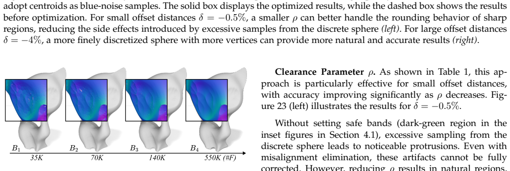
- Sharp features are treated by a one-base-many-displaced sampling around edges and vertices, and by restricting the allowed displacement directions the method can also produce feature-preserved or topology-changing offsets, such as in dilation-erosion closing operations.
Reading between the lines
- Extension: the same weighted-site construction should work for radius functions defined on point clouds or implicit surfaces, provided one can estimate a gradient and a normal field; the paper demonstrates only triangle-mesh inputs.
- Testable consequence: as sampling density grows and $\epsilon\to 0$, the least-squares fix should make the extracted facets converge to the true zero level set; an experiment varying only sample count would show whether residual error comes from sampling or from the offset-direction approximation.
- The method's sharp-feature fidelity depends on the heuristic spherical interpolation between face-based displacement directions, so varying the dihedral-angle threshold at fixed sample count would isolate the contribution of Theorem 1 from the contribution of the sampling heuristic.
- The MAT application suggests a stress test: feed in a medial axis with a radius field that locally violates $\|\nabla R\|\le 1$, such as near a crease, and check whether the unresolvable misalignments predicted by the paper appear exactly where the constraint fails.
Editorial analysis
A structured set of objections, weighed in public.
Referee Report
Summary. The paper proposes OffsetCrust, a crust-based method for approximating variable-radius offset surfaces of triangle meshes. Given a radius function R on a base surface S, it samples base points p with power weight R(p)^2 and displaced points p_R^epsilon = p + epsilon n_R^off(p) with weight (R(p)-epsilon)^2, then extracts the offset as the subset of power diagram facets separating base and displaced sites. The displacement direction n_R^off is claimed to be the surface normal rotated by arcsin(||grad R||) around an axis determined by grad R and n_p (Theorem 1). A least-squares refinement moves power diagram vertices to reduce misaligned facets. The method is validated quantitatively on a Dupin cyclide, qualitatively on CAD and freeform models, and on 7,609 Thingi10K meshes for the constant-radius case; applications include expressive surface design, channel surfaces, and MAT reconstruction.
Significance. If the central identity is correct, the paper offers a novel and efficient way to compute variable-radius offsets without explicit self-intersection handling, with a clean geometric interpretation via power diagrams. Strengths include the simple formulation, the large-scale constant-radius evaluation on Thingi10K, and the public code release. The method also enables interesting extensions such as feature-preserving offsets by restricting displacement directions. However, the load-bearing derivation of the displacement direction is only sketched, and some strong topological claims are contradicted by the paper's own appendix statistics; these issues need to be fixed before the contribution is fully established.
major comments (3)
- [§3.2, Theorem 1 / Figure 3] The displacement direction n_R^off is the single most load-bearing quantity in the paper: every displaced site, every power facet, and the misalignment objective in Eq. (14) depend on it. Yet the proof of Theorem 1 is only a verbal description of a right triangle; it does not derive the triangle from the stationarity condition of Eq. (1), does not state whether n_p is the inward or outward normal, and does not handle the piecewise-linear case where grad R is per-face and undefined on edges and vertices. The correct smooth-surface identity is that the tangent component of n_R^off equals -grad_S R(p), i.e., n_R^off = sqrt(1-||grad R||^2) n_p - grad R(p) for an outward offset, with the sign of the normal component reversed for an inward offset. The rotation formula in Theorem 1 is consistent with this identity, but the text never establishes it. I ask the authors to replace the diagram-based argument with a derivation from Eq. (1) and to state explicitly how the edge/vertex Slerp and 1vN heuristics in §4.1 relate to this continuous formula.
- [§3.2 'Manifold Output...' vs Appendix E, Table 3] The subsection titled 'Manifold Output Without the Need for Explicit Self-Intersection Handling' claims that non-manifoldness cannot occur. This is contradicted by the authors' own Appendix E statistics: for delta = -2% with the optimized pipeline, Table 3 reports mean non-manifold edge proportion 0.002% (max 0.376%), mean non-manifold vertex proportion 0.023% (max 0.398%), and mean non-coplanar intersecting face proportion 11.759% (max 66.176%). Even the raw output has up to 5.128% intersecting faces for delta = -2%. The claim should be corrected to state that non-manifold and self-intersecting artifacts are rare but not eliminated by construction, especially after the misalignment optimization.
- [§5.1-5.2] The quantitative validation of the central variable-radius claim is thin. The only quantitative variable-radius evaluation is on the Dupin cyclide (§5.1.1), a single smooth analytical surface. The Thingi10K large-scale evaluation in §5.2 is for constant-radius offsets (delta = ±2%) only, and the qualitative comparisons in §5.1.2 do not report error metrics against a ground truth. Since the method's novelty is precisely the variable-radius case, I would like to see at least a few quantitative variable-radius tests on triangle meshes, for example by comparing against a high-resolution sampled version of Eq. (1) or against offset spheres/cones/slabs for models with known radius functions.
minor comments (6)
- [§3.2, Theorem 1] The theorem statement uses grad R(p) without specifying that it is the surface (tangential) gradient; in the discrete setting R is piecewise linear per triangle, so grad R is not defined on edges and vertices. Please make this distinction explicit.
- [§5.2] The sentence 'the NC metric exhibits significant improvement, improving by approximately an order of magnitude' is imprecise because NC values are percentages near 100%; please report the actual before/after values or clarify what 'order of magnitude' refers to.
- [Table 1] The formatting of bold entries is confusing because both the best and second-best scores are marked in bold; some cells also appear to run together. Please reformat the table so the best and second-best scores are visually distinguishable.
- [§4.1] Several inset figures are referenced without numbers, which hurts readability. Please number the insets for the edge-type, vertex-type, and cylinder-based sampling strategies.
- [Appendix A] The notation d_pow(x, p_i) is used in Eqs. (19)-(26) without being redefined in the appendix; please add a pointer to Eq. (6) so the appendix is self-contained.
- [References] Reference [31] is cited as 'Qun et al.' but the paper is by Qun and Rokne; please correct the citation style.
Circularity Check
No circularity: the offset is defined externally by Eq. (1), the power-diagram weights are chosen so that bisectors coincide with tangent planes at true offset points, the displacement direction comes from ∇R via Theorem 1 rather than from the output, and accuracy is checked against analytical and distance-field ground truth.
full rationale
The derivation chain is self-contained. The offset surface is fixed by Eq. (1), φ(x) = min_{p∈S}( ‖x−p‖ − R(p) ) = 0, which never references the power diagram. The weighted-site construction is an engineering identity, not a prediction: Eq. (3)-(4) ('‖p_off_R − p‖ − R(p) = ‖p_off_R − p_eps_R‖ − (R(p) − ε) = 0', 'or equivalently' the squared form) hold because the weights R(p)² and (R(p) − ε)² are chosen so that the bisector plane between p and p_eps_R passes through p_off_R and is perpendicular to n_off_R(p); the bisector is the tangent plane of the true offset only if n_off_R(p) is the true displacement direction. That direction is not fitted: Theorem 1 (rotating the unit normal n_p by α = arcsin(‖∇R(p)‖) around ∇R/‖∇R‖ × n_p) uses only R and the surface geometry. Its proof in Section 3.2 is a sketch (a right triangle with hypotenuse ‖pq‖ and leg |R(p) − R(q)|) and is under-specified for piecewise-linear meshes, but an under-proved identity is a rigor gap, not circularity; the paper's own Section 7 explicitly concedes the arcsin domain restriction ‖∇R‖ ≤ 1 and the heuristic design of the face/edge/vertex sampling strategies. Validation is external: the Dupin cyclide analytical ground truth (Section 5.1.1), projection-distance error against the original surface for constant offsets (Section 5), comparisons with PointDC, which builds the distance field directly from Eq. (1) (Section 5.1.2), and MAT reconstruction measured against the original boundary surfaces (Section 6.3). The misalignment elimination (Eq. 14-15) minimizes (v − p_i)·n_off_i − d_i with d_i := R(p_i), i.e., the input radius, not a measured target, and the reported Normal Consistency gains are computed against external normals, so the fine-tuning is not a disguised fit to the expected answer. Self-citations (PCO [14], Q-MAT [52]) serve only as a comparison baseline and as a generator of MAT test inputs; neither justifies a load-bearing premise. No uniqueness theorem is imported from the authors' prior work, and the weighted-site ansatz is derived in-paper from Eq. (4) rather than adopted via citation. Accordingly, no specific circular reduction can be quoted, and the score is 0.
Assumptions & free parameters
free parameters (7)
- epsilon (displacement distance) =
1e-6
- lambda (regularization weight) =
0.01
- rho (clearance parameter) =
5% of average edge length
- blue-noise sample count =
70,000
- vertex sphere discretization =
642 vertices
- dihedral angle threshold =
0.2 rad
- TetWild preprocessing edge length =
0.5
assumptions (6)
- domain assumption Input meshes are watertight, free of self-intersections, and have good triangle quality.
- domain assumption The radius function R is smooth with ||grad R(p)|| <= 1 everywhere.
- domain assumption The power diagram is generic: no more than three sites determine a vertex in 2D and four in 3D.
- domain assumption If a point p does not contribute to the offset, there exists another point q whose ball strictly contains p_R^off.
- domain assumption The proof of Theorem 1 treats pq, |R(p)-R(q)|, and the tangent-plane leg as a right triangle, which holds to first order only for smooth surfaces and smooth R.
- standard math Power diagram properties and weighted distance geometry from Aurenhammer (1987).
invented entities (1)
-
paired power diagram sites (base point p with weight R(p)^2 and displaced point p_R^eps with weight (R(p)-eps)^2)
Cite this review
Pith. "Pith review of OffsetCrust: Variable-Radius Offset Approximation with Power Diagrams." pith.science (2026). https://pith.science/paper/HTOGS4YF
@misc{pith2026250710924,
  author       = {Pith},
  title        = {Pith review of: OffsetCrust: Variable-Radius Offset Approximation with Power Diagrams},
  year         = {2026},
  howpublished = {\url{https://pith.science/paper/HTOGS4YF}},
  note         = {Machine review of arXiv:2507.10924}
}
abstract
Offset surfaces, defined as the Minkowski sum of a base surface and a rolling ball, play a crucial role in geometry processing, with applications ranging from coverage motion planning to brush modeling. While considerable progress has been made in computing constant-radius offset surfaces, computing variable-radius offset surfaces remains a challenging problem. In this paper, we present OffsetCrust, a novel framework that efficiently addresses the variable-radius offsetting problem by computing a power diagram. Let $R$ denote the radius function defined on the base surface $S$. The power diagram is constructed from contributing sites, consisting of carefully sampled base points on $S$ and their corresponding off-surface points, displaced along $R$-dependent directions. In the constant-radius case only, these displacement directions align exactly with the surface normals of $S$. Moreover, our method mitigates the misalignment issues commonly seen in crust-based approaches through a lightweight fine-tuning procedure. We validate the accuracy and efficiency of OffsetCrust through extensive experiments, and demonstrate its practical utility in applications such as reconstructing original boundary surfaces from medial axis transform (MAT) representations.
Figures


Figures from the paper (26 more)






Reference graph
Works this paper leans on
-
[1]
Offsetting operations in solid modelling,
J. R. Rossignac and A. A. Requicha, “Offsetting operations in solid modelling,”Computer Aided Geometric Design, vol. 3, no. 2, pp. 129– 148, 1986
work page 1986
-
[2]
Robot motion planning in a dynamic environment using offset non- uniform rational b-splines (nurbs),
A. K. Singh, A. Aggarwal, M. Vashisht, and R. Siddavatam, “Robot motion planning in a dynamic environment using offset non- uniform rational b-splines (nurbs),” in2011 IEEE International Conference on Industrial Technology. IEEE, 2011, pp. 312–317
work page 2011
-
[3]
Weighted skeletal structures for com- puting variable-radius offsets,
M. Held and S. De Lorenzo, “Weighted skeletal structures for com- puting variable-radius offsets,”Comput. Aided Des. Appl, vol. 18, pp. 875–889, 2021
work page 2021
-
[4]
Marching cubes: A high res- olution 3d surface construction algorithm,
W. E. Lorensen and H. E. Cline, “Marching cubes: A high res- olution 3d surface construction algorithm,” inSeminal graphics: pioneering efforts that shaped the field, 1998, pp. 347–353
work page 1998
-
[5]
Marching cubes 33: Construction of topologically correct isosurfaces,
E. Chernyaev, “Marching cubes 33: Construction of topologically correct isosurfaces,” Tech. Rep., 1995
work page 1995
-
[6]
Dual contouring of hermite data,
T. Ju, F. Losasso, S. Schaefer, and J. Warren, “Dual contouring of hermite data,” inProceedings of the 29th annual conference on Computer graphics and interactive techniques, 2002, pp. 339–346
work page 2002
-
[7]
G. M. Nielson, “Dual marching cubes,” inIEEE visualization 2004. IEEE, 2004, pp. 489–496
work page 2004
-
[8]
Half-space power diagrams and discrete surface offsets,
Z. Chen, D. Panozzo, and J. Dumas, “Half-space power diagrams and discrete surface offsets,”IEEE Transactions on Visualization and Computer Graphics, vol. 26, no. 10, pp. 2970–2981, 2019
work page 2019
Show all 54 references
-
[9]
Neural marching cubes,
Z. Chen and H. Zhang, “Neural marching cubes,”ACM Transac- tions on Graphics (TOG), vol. 40, no. 6, pp. 1–15, 2021
2021
-
[10]
Neural dual contouring,
Z. Chen, A. Tagliasacchi, T. Funkhouser, and H. Zhang, “Neural dual contouring,”ACM Transactions on Graphics (TOG), vol. 41, no. 4, pp. 1–13, 2022
2022
-
[11]
An efficient method of triangulating equi- valued surfaces by using tetrahedral cells,
A. Doi and A. Koide, “An efficient method of triangulating equi- valued surfaces by using tetrahedral cells,”IEICE TRANSAC- TIONS on Information and Systems, vol. 74, no. 1, pp. 214–224, 1991
1991
-
[12]
Regularised marching tetrahedra: improved iso-surface extraction,
G. M. Treece, R. W. Prager, and A. H. Gee, “Regularised marching tetrahedra: improved iso-surface extraction,”Computers & Graph- ics, vol. 23, no. 4, pp. 583–598, 1999
1999
-
[13]
Deep march- ing tetrahedra: a hybrid representation for high-resolution 3d shape synthesis,
T. Shen, J. Gao, K. Yin, M.-Y. Liu, and S. Fidler, “Deep march- ing tetrahedra: a hybrid representation for high-resolution 3d shape synthesis,”Advances in Neural Information Processing Systems, vol. 34, pp. 6087–6101, 2021
2021
-
[14]
Pco: Precision-controllable offset surfaces with sharp features,
L. Wang, X. Wang, P . Wang, S. Chen, S. Xin, J. Guo, W. Wang, and C. Tu, “Pco: Precision-controllable offset surfaces with sharp features,”ACM Transactions on Graphics (TOG), vol. 43, no. 6, pp. 1–16, 2024
2024
-
[15]
Feature- preserving offset mesh generation from topology-adapted oc- trees,
D. Zint, N. Maruani, M. Rouxel-Labb, and P . Alliez, “Feature- preserving offset mesh generation from topology-adapted oc- trees,” inComputer Graphics Forum, vol. 42, no. 5. Wiley Online Library, 2023, p. e14906
2023
-
[16]
Comparing offset curve approximation methods,
G. Elber, I.-K. Lee, and M.-S. Kim, “Comparing offset curve approximation methods,”IEEE computer graphics and applications, vol. 17, no. 3, pp. 62–71, 1997
1997
-
[17]
An overview of offset curves and surfaces,
T. Maekawa, “An overview of offset curves and surfaces,” Computer-Aided Design, vol. 31, no. 3, pp. 165–173, 1999
1999
-
[18]
Offset curves and surfaces: a brief survey,
B. Pham, “Offset curves and surfaces: a brief survey,”Computer- Aided Design, vol. 24, no. 4, pp. 223–229, 1992
1992
-
[19]
Approximation of variable- radius offset curves and its application to b ´ezier brush-stroke design,
M.-S. Kim, E.-J. Park, and S.-B. Lim, “Approximation of variable- radius offset curves and its application to b ´ezier brush-stroke design,”Computer-Aided Design, vol. 25, no. 11, pp. 684–698, 1993
1993
-
[20]
Self- intersections of offset curves and surfaces,
J. Wallner, T. Sakkalis, T. Maekawa, H. Pottmann, and G. Yu, “Self- intersections of offset curves and surfaces,”International Journal of Shape Modeling, vol. 7, no. 01, pp. 1–21, 2001
2001
-
[21]
A gpu-based voxelization approach to 3d minkowski sum computation,
W. Li and S. McMains, “A gpu-based voxelization approach to 3d minkowski sum computation,” inProceedings of the 14th ACM symposium on solid and physical modeling, 2010, pp. 31–40
2010
-
[22]
A sweep and translate algorithm for computing voxelized 3d minkowski sums on the gpu,
——, “A sweep and translate algorithm for computing voxelized 3d minkowski sums on the gpu,”Computer-Aided Design, vol. 46, pp. 90–100, 2014
2014
-
[23]
Voxelized minkowski sum computation on the gpu with robust culling,
——, “Voxelized minkowski sum computation on the gpu with robust culling,”Computer-Aided Design, vol. 43, no. 10, pp. 1270– 1283, 2011
2011
-
[24]
Real-time shaded nc milling display,
T. Van Hook, “Real-time shaded nc milling display,”ACM SIG- GRAPH Computer Graphics, vol. 20, no. 4, pp. 15–20, 1986
1986
-
[25]
Feature preserving distance fields,
H. Qu, N. Zhang, R. Shao, A. Kaufman, and K. Mueller, “Feature preserving distance fields,” in2004 IEEE Symposium on Volume Visualization and Graphics. IEEE, 2004, pp. 39–46
2004
-
[26]
High-resolution volumetric computation of offset surfaces with feature preservation,
D. Pavi ´c and L. Kobbelt, “High-resolution volumetric computation of offset surfaces with feature preservation,” inComputer Graphics Forum, vol. 27, no. 2. Wiley Online Library, 2008, pp. 165–174
2008
-
[27]
A robust and efficient implementation for the segment voronoi diagram,
M. Karavelas, “A robust and efficient implementation for the segment voronoi diagram,”International Symposium on Voronoi Diagrams in Science and Engineering, 01 2004
2004
-
[28]
Held,On the computational geometry of pocket machining
M. Held,On the computational geometry of pocket machining. Springer Science & Business Media, 1991, vol. 500
1991
-
[29]
Generalized offsetting of planar structures using skeletons,
M. Held, S. Huber, and P . Palfrader, “Generalized offsetting of planar structures using skeletons,”Computer-Aided Design and Applications, vol. 13, no. 5, pp. 712–721, 2016
2016
-
[30]
Point morphology,
S. Calderon and T. Boubekeur, “Point morphology,”ACM Transac- tions on Graphics (TOG), vol. 33, no. 4, pp. 1–13, 2014
2014
-
[31]
Variable-radius offset curves and surfaces,
L. Qun and J. Rokne, “Variable-radius offset curves and surfaces,” Mathematical and Computer Modelling, vol. 26, no. 7, pp. 97–108, 1997
1997
-
[32]
Variable-radius offset surface approximation on the gpu,
A.-C. Woerl, E. Schoemer, and U. Schwanecke, “Variable-radius offset surface approximation on the gpu,” 2020
2020
-
[33]
Robust and feature-preserving offset meshing,
H. Cao, G. Xu, R. Gu, J. Xu, X. Zhang, T. Rabczuk, Y. Luo, and X. Gao, “Robust and feature-preserving offset meshing,”arXiv preprint arXiv:2412.15564, 2024
2024 arXiv
-
[34]
Topological offsets,
D. Zint, Z. Chen, Y. Zhu, D. Zorin, T. Schneider, and D. Panozzo, “Topological offsets,”ACM Transactions on Graphics (TOG), vol. 44, no. 4, pp. 1–19, 2025
2025
-
[35]
The power crust,
N. Amenta, S. Choi, and R. K. Kolluri, “The power crust,” in Proceedings of the sixth ACM symposium on Solid modeling and applications, 2001, pp. 249–266
2001
-
[36]
Vorocrust: Voronoi meshing without clipping,
A. Abdelkader, C. L. Bajaj, M. S. Ebeida, A. H. Mahmoud, S. A. Mitchell, J. D. Owens, and A. A. Rushdi, “Vorocrust: Voronoi meshing without clipping,”ACM Transactions on Graphics (TOG), vol. 39, no. 3, pp. 1–16, 2020
2020
-
[37]
Sampling conditions for conforming voronoi meshing by the vorocrust algorithm,
——, “Sampling conditions for conforming voronoi meshing by the vorocrust algorithm,”LIPIcs: Leibniz international proceedings in informatics, vol. 99, 2018
2018
-
[38]
Power diagrams: properties, algorithms and applications,
F. Aurenhammer, “Power diagrams: properties, algorithms and applications,”SIAM Journal on Computing, vol. 16, no. 1, pp. 78– 96, 1987. [39]CGAL User and Reference Manual: Tri- angulation, CGAL Editorial Board, 2024, https://doc.cgal.org/latest/Triangulation/index.html
1987
-
[40]
Surface simplification using quadric error metrics,
M. Garland and P . S. Heckbert, “Surface simplification using quadric error metrics,” inProceedings of the 24th annual conference on Computer graphics and interactive techniques, 1997, pp. 209–216
1997
-
[41]
CGAL Editorial Board, 2024
The CGAL Project,CGAL User and Reference Manual, 5.6.1 ed. CGAL Editorial Board, 2024. [Online]. Available: https://doc. cgal.org/5.6.1/Manual/packages.html
2024
-
[42]
Intel® threading building blocks,
C. Pheatt, “Intel® threading building blocks,”Journal of Computing Sciences in Colleges, vol. 23, no. 4, pp. 298–298, 2008
2008
-
[43]
Eigen v3,
G. Guennebaud, B. Jacobet al., “Eigen v3,” http://eigen.tuxfamily.org, 2010
2010
-
[44]
Openmp: an industry standard api for shared-memory programming,
L. Dagum and R. Menon, “Openmp: an industry standard api for shared-memory programming,”Computational Science & Engineer- ing, IEEE, vol. 5, no. 1, pp. 46–55, 1998
1998
-
[45]
Fast proxim- ity queries with swept sphere volumes,
E. Larsen, S. Gottschalk, M. C. Lin, and D. Manocha, “Fast proxim- ity queries with swept sphere volumes,” Technical Report TR99- 018, Department of Computer Science, University of . . . , Tech. Rep., 1999
1999
-
[46]
libigl: A simple C++ geometry processing library,
A. Jacobson, D. Panozzoet al., “libigl: A simple C++ geometry processing library,” 2018, https://libigl.github.io/. 13
2018
-
[47]
Tetrahedral meshing in the wild
Y. Hu, Q. Zhou, X. Gao, A. Jacobson, D. Zorin, and D. Panozzo, “Tetrahedral meshing in the wild.”ACM Trans. Graph., vol. 37, no. 4, p. 60, 2018
2018
-
[48]
Fast tetrahedral meshing in the wild,
Y. Hu, T. Schneider, B. Wang, D. Zorin, and D. Panozzo, “Fast tetrahedral meshing in the wild,”ACM Trans. Graph., vol. 39, no. 4, Jul. 2020
2020
-
[49]
Abc: A big cad model dataset for geometric deep learning,
S. Koch, A. Matveev, Z. Jiang, F. Williams, A. Artemov, E. Burnaev, M. Alexa, D. Zorin, and D. Panozzo, “Abc: A big cad model dataset for geometric deep learning,” inThe IEEE Conference on Computer Vision and Pattern Recognition (CVPR), June 2019
2019
-
[50]
Thingi10k: A dataset of 10,000 3d- printing models,
Q. Zhou and A. Jacobson, “Thingi10k: A dataset of 10,000 3d- printing models,” 2016
2016
-
[51]
Computing rational parametriza- tions of canal surfaces,
M. Peternell and H. Pottmann, “Computing rational parametriza- tions of canal surfaces,”Journal of Symbolic Computation, vol. 23, no. 2-3, pp. 255–266, 1997
1997
-
[52]
Q-mat: Computing medial axis transform by quadratic error minimiza- tion,
P . Li, B. Wang, F. Sun, X. Guo, C. Zhang, and W. Wang, “Q-mat: Computing medial axis transform by quadratic error minimiza- tion,”ACM Transactions on Graphics (TOG), vol. 35, no. 1, pp. 1–16, 2015
2015
-
[53]
Computing medial axis transform with feature preservation via restricted power diagram,
N. Wang, B. Wang, W. Wang, and X. Guo, “Computing medial axis transform with feature preservation via restricted power diagram,”ACM Transactions on Graphics (TOG), vol. 41, no. 6, pp. 1–18, 2022
2022
-
[54]
Mat- topo: Topology-preserving medial axis transform with restricted power diagram,
N. Wang, H. Huang, S. Song, B. Wang, W. Wang, and X. Guo, “Mat- topo: Topology-preserving medial axis transform with restricted power diagram,”ACM Transactions on Graphics (TOG), vol. 43, no. 4, 2024
2024
-
[55]
Triangulation by ear clipping,
D. Eberly, “Triangulation by ear clipping,”Geometric Tools, pp. 2002–2005, 2008. APPENDIXA ANALYSIS OFMISALIGNEDFACETS Based on Section 3.2, we can filter the offset facets. However, due to the discontinuities in real sampling, some additional facets are also included to prese...
2002
Reviewed August 6, 2026 · model on record in the stance chip above.
Discussion (0). Sign in to comment.