REVIEW 3 major objections 6 minor 25 references
Physics-Informed Transfer Learning for Data-Driven Sound Source Reconstruction in Near-Field Acoustic Holography
T0 review · 3 major / 6 minor · reviewed 2026-08-06 · deepseek-v4-flash
Pith's one-line read Fine-tuning a pre-trained network on a single violin sample with a physics-based loss—instead of ground-truth labels—reconstructs source velocity as accurately as the Compressive Equivalent Source Method, and outperforms it on the modes…
desk verdict A modest but real transfer-learning result for NAH: single-sample physics-informed fine-tuning improves over the pre-trained model and lands near C-ESM, but the paper under-specifies its forward model and overreaches on a post hoc 'successful modes' claim. read the letter →
The pith
A machine-rendered reading of the paper's core claim, the machinery that carries it, and where it could break.
The reading
What carries the argument
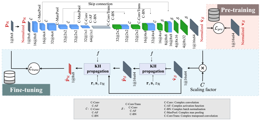
The workhorse is the complex-valued U-Net (CV-CNN) that maps hologram pressure to source velocity, pre-trained with an MSE velocity loss and fine-tuned with a mean-absolute-error physics loss. The physics loss is load-bearing: it computes predicted hologram pressure by forward-propagating the network's predicted velocity through the discrete Kirchhoff-Helmholtz integral (Eq. 1) and compares it to the measured pressure. A trainable scalar rescales the normalized network output to physical units. The paper uses the pre-trained weights as the initialization for fine-tuning and a small learning rate to keep the network close to that initialization, arguing this avoids the non-uniqueness of direct source-plane inversion.
What would settle it
Re-run the fine-tuning with the surface-pressure term of Eq. (1) explicitly included, using measured or equivalent-source pressure, or alternatively compare against a fine-tuned model whose physics loss replaces the KH forward model by a free-form linear propagator; if the published NMSE and NCC values do not change materially, the physics content of the loss is not what produced the reported gains.
Extended reading notes
Core claim
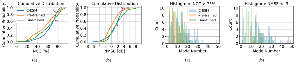
The central claim is that the self-supervised fine-tuning step, not the architecture or the supervision, transfers the source reconstruction capability. The paper states that a pre-trained CV-CNN, initialized from a rectangular-plate dataset and further trained for 2000 epochs on a single violin top-plate sample with the loss of Eq. (6), reproduces the normal surface velocity with an average NMSE of -1.76 dB and NCC of 60.66%, compared with -0.33 dB and 54.52% for the unadapted pre-trained network and -1.13 dB and 63.20% for C-ESM. In the cumulative-distribution analysis, the fine-tuned model and C-ESM cross; above the crossing (the successful modes), the fine-tuned model is more accurate. The paper also claims that a randomly initialized model trained on the same physics loss fails due to non-uniqueness and singularity, which is why the pre-trained initialization is essential.
Load-bearing premise
The fine-tuning loss assumes that the predicted hologram pressure can be computed from the predicted source velocity alone, but the stated Kirchhoff-Helmholtz integral also contains a surface-pressure term that the paper never says how it handles; if that term is silently dropped, the physics loss is enforcing an incomplete forward model.
Editorial extensions
If this is right
- A model pre-trained on a cheap, abundant simulation domain can be reused for a scarce, geometrically different target without any target-side ground-truth velocity labels.
- Because fine-tuning costs about 1.28 minutes per sample versus 4.09 hours of pre-training, per-instance adaptation is fast enough to consider for real-world NAH applications.
- The method's accuracy is concentrated at low mode numbers; high-frequency violin modes are where both the pre-trained and fine-tuned models fall behind C-ESM.
- On modes with NCC above 75%, the fine-tuned model outperforms both the pre-trained network and C-ESM, suggesting the physics prior and the learned prior are complementary.
Reading between the lines
- Beyond the paper: we infer the same two-stage recipe should transfer across other source pairs, such as from a simulated box to a car panel or loudspeaker cabinet, wherever a proxy geometry can be simulated in bulk; the paper demonstrates only rectangular plates to violin top plates.
- The paper leaves the forward model's treatment of the surface-pressure term in Eq. (1) unspecified; a testable extension is to run the fine-tuning with the full integral including the surface pressure to see whether the reported gains survive.
- An implication the authors do not draw: the physics loss acts as a regularizer that substitutes for labeled target data, so the approach predicts that a single sample is sufficient; this could be probed by fine-tuning on 1, 2, 5, and 10 samples and measuring whether accuracy saturates.
Editorial analysis
A structured set of objections, weighed in public.
Referee Report
Summary. The paper proposes a two-stage transfer-learning framework for near-field acoustic holography (NAH). In the first stage, a complex-valued U-Net (CV-CNN) is pretrained on simulated rectangular-plate data using a supervised MSE loss on the source velocity. In the second stage, the network is fine-tuned on a single violin-top-plate sample using a physics-informed MAE loss (Eq. 6) that compares the measured hologram pressure with a pressure field computed from the predicted source velocity through the Kirchhoff-Helmholtz integral. The authors report that fine-tuning improves NMSE and NCC relative to the pretrained model, achieves performance comparable to the Compressive-Equivalent Source Method (C-ESM), and, for a selected subset of 'successful modes,' outperforms both baselines. The paper includes cumulative distribution plots, a random-initialization sanity check, and per-mode histograms to support the analysis.
Significance. If the claims hold, the core idea is valuable: adapting a data-driven NAH model to a new source geometry using a single unlabeled sample and a physics-based loss would address a real limitation of supervised deep-learning approaches, namely poor out-of-distribution generalization. The two-stage design is attractive because it avoids backpropagation through the integral operator during pretraining, and the comparison with C-ESM is a useful benchmark. The paper also includes a reasonable amount of experimental detail (dataset splits, optimizer settings, metrics, and runtime). However, the significance is conditional on resolving two load-bearing issues: the exact forward model used in the physics loss is not specified completely, and the reported accuracy is evaluated on the same samples used for fine-tuning rather than on held-out data. The post hoc selection of 'successful modes' also weakens the strongest comparative claims.
major comments (3)
- [Sec. 3, Eqs. (1) and (6)] The text states that the fine-tuning loss computes pH using the Kirchhoff-Helmholtz integral of Eq. (1) from the predicted source velocity. However, Eq. (1) contains two surface integrals: one involving the surface pressure p(s,ω) and one involving the normal velocity vn(s,ω). The network output, Eq. (4), provides only vS, and the paper never states how p(s) is obtained, approximated, or assumed to vanish. If the implemented forward model is a velocity-only Rayleigh-type integral (or a precomputed propagation matrix that drops the pressure term), then for an unbaffled violin top plate the loss in Eq. (6) does not enforce the stated KH integral, and the claim that the fine-tuning is 'physics-informed' in the sense of Eq. (1) is unsupported. The authors must specify the exact discrete forward operator used to compute pH, including any baffle assumption, and justify its validity for the unbaffled geometry, or modify the loss to include the missing surface-pressure contribution.
- [Sec. 4.2, Table 1 and Fig. 3] The fine-tuning loss is optimized on the same sample for which the reconstruction accuracy is then reported. Consequently, the NMSE and NCC values in Table 1 are fitting accuracies rather than held-out generalization metrics. This matters because the contribution is framed as adapting to new data with limited labels; an in-sample evaluation cannot distinguish genuine physical adaptation from overfitting to the measured pressure. Even for a per-sample inverse problem, the authors should report a consistency check (e.g., forward residual on independent pressure points or modes) and compare against a direct pressure-fitting baseline that does not use the pretrained initialization, to demonstrate what the physics-informed fine-tuning adds beyond solving the inverse problem from scratch.
- [Sec. 4.2, Fig. 4] The category of 'successful modes' is defined by thresholds (NCC > 75%, NMSE < -3) that appear to be chosen after seeing the results, and the conclusion that the fine-tuned model outperforms C-ESM and the pretrained model is drawn only on this selected subset. This is a post hoc selection on the outcome, which inflates the strength of the comparative claim. The authors should either specify these thresholds a priori, or present the full distributions without selection and discuss threshold sensitivity, or use a proper multiple-testing correction when reporting success counts across modes.
minor comments (6)
- [Abstract and Sec. 3] The phrase 'purely physics-informed fine-tuning' is slightly misleading because the loss in Eq. (6) also uses measured pressure pH, and a trainable scaling factor C is introduced; 'purely' could be replaced by 'data-free with respect to the source velocity' or a similar qualification.
- [Sec. 4.2, text near Fig. 3] The explanation that NMSE is accumulated in descending order to align with NCC trends is hard to follow; a more standard definition of the cumulative distribution or a direct plot of P(NMSE <= x) would improve clarity.
- [Sec. 4.1] It is stated that fine-tuning is performed for all modes on 10 different violin top plates (442 samples in total), but it is not clear how many modes per plate are included and whether the reported means in Table 1 are over samples, modes, or both; reporting standard deviations or per-mode details would help.
- [Throughout, Eq. (7)] The symbol H is used both for the hologram plane and for the Hermitian transpose operator in Eq. (7); this notational collision is confusing and should be resolved, for example by using the dagger symbol.
- [Table 1] The runtime for C-ESM is left as a hyphen; if the implementation time is unavailable, a qualitative statement about computational cost would be preferable to an empty cell.
- [Sec. 2.1] 'The eigenfrequency for the dataset generation is limited' should be rephrased as 'the eigenfrequencies are limited' or 'the natural frequencies are limited,' and the sentence appears in Sec. 4.1 rather than Sec. 2.1 in the submitted text.
Circularity Check
No circular derivation: the physics-informed fine-tuning loss is not identical to the reported velocity metric, and the C-ESM benchmark provides independent grounding.
full rationale
The claimed chain is: pre-train a CV-CNN on rectangular plates, then fine-tune it on a single violin sample by matching hologram pressure via a KH-based forward model, then evaluate reconstructed velocity against ground truth. No step in this chain equates an input to an output by construction. The fine-tuning loss (Eq. 6) fits measured pressure pH, not the ground-truth velocity vS; the reported NMSE/NCC are computed against vS, so the improvement is an empirical result rather than a fitted parameter renamed as a prediction. The random-initialization experiment (Fig. 2e,j) further shows that the pressure loss alone does not force the velocity solution, so the success of the fine-tuned model is not a tautology. The comparisons with C-ESM, an external baseline, provide independent support. Self-citations to [3]-[5] supply architecture, dataset, and loss-design choices, but the pre-training is rerun here and the benchmark is external, so the self-citations are not load-bearing reductions. One substantive gap exists: the paper states that p̂H is computed via the KH integral (Eq. 1) from the predicted source velocity, yet Eq. 1 contains a surface-pressure term p(s,ω) that the network does not output and the paper never explains how it is obtained or omitted; however, this is an under-specification of the forward model and a correctness risk, not a circularity in the derivation chain.
Assumptions & free parameters
free parameters (1)
- scaling factor C =
trainable, not reported
assumptions (4)
- domain assumption The Kirchhoff-Helmholtz integral is the correct forward model for the pressure field.
- ad hoc to paper The hologram pressure can be computed from the predicted normal velocity alone, without the surface pressure term in Eq. (1).
- domain assumption Pre-trained network weights provide a regularization prior that avoids non-uniqueness and singularity in direct source-plane inversion.
- domain assumption The simulated dataset from [3] is representative of real plate and violin top plate vibrations.
Cite this review
Pith. "Pith review of Physics-Informed Transfer Learning for Data-Driven Sound Source Reconstruction in Near-Field Acoustic Holography." pith.science (2026). https://pith.science/paper/5P723O5H
@misc{pith2026250711070,
  author       = {Pith},
  title        = {Pith review of: Physics-Informed Transfer Learning for Data-Driven Sound Source Reconstruction in Near-Field Acoustic Holography},
  year         = {2026},
  howpublished = {\url{https://pith.science/paper/5P723O5H}},
  note         = {Machine review of arXiv:2507.11070}
}
read the original abstract
We propose a transfer learning framework for sound source reconstruction in Near-field Acoustic Holography (NAH), which adapts a well-trained data-driven model from one type of sound source to another using a physics-informed procedure. The framework comprises two stages: (1) supervised pre-training of a complex-valued convolutional neural network (CV-CNN) on a large dataset, and (2) purely physics-informed fine-tuning on a single data sample based on the Kirchhoff-Helmholtz integral. This method follows the principles of transfer learning by enabling generalization across different datasets through physics-informed adaptation. The effectiveness of the approach is validated by transferring a pre-trained model from a rectangular plate dataset to a violin top plate dataset, where it shows improved reconstruction accuracy compared to the pre-trained model and delivers performance comparable to that of Compressive-Equivalent Source Method (C-ESM). Furthermore, for successful modes, the fine-tuned model outperforms both the pre-trained model and C-ESM in accuracy.
Figures

Reference graph
Works this paper leans on
-
[1]
Near- field acoustic holography analysis with convolutional neural networks,
M. Olivieri, M. Pezzoli, R. Malvermi, F. Antonacci, and A. Sarti, “Near- field acoustic holography analysis with convolutional neural networks,” in INTER-NOISE and NOISE-CON Congress and Conference Proceedings , vol. 261, no. 1. Institute of Noise Control Engineering, 2020, pp. 5607–5618
work page 2020
-
[2]
Near field acoustic holography on arbitrary shapes using convolutional neural network,
M. Olivieri, M. Pezzoli, F. Antonacci, and A. Sarti, “Near field acoustic holography on arbitrary shapes using convolutional neural network,” in 2021 29th European Signal Processing Conference (EUSIPCO) . IEEE, 2021, pp. 121–125
work page 2021
-
[3]
A physics-informed neural network approach for nearfield acoustic holography,
M. Olivieri, M. Pezzoli, F. Antonacci, and A. Sarti, “A physics-informed neural network approach for nearfield acoustic holography,” Sensors, vol. 21, no. 23, p. 7834, 2021
work page 2021
-
[4]
Complex- valued physics-informed neural network for near-field acoustic hologra- phy,
X. Luan, M. Olivieri, M. Pezzoli, F. Antonacci, and A. Sarti, “Complex- valued physics-informed neural network for near-field acoustic hologra- phy,” in 2024 32nd European Signal Processing Conference (EUSIPCO) . IEEE, 2024, pp. 126–130
work page 2024
-
[5]
X. Luan, M. Pezzoli, F. Antonacci, and A. Sarti, “Physics-informed neural network-driven sparse field discretization method for near-field acoustic holography,” arXiv preprint arXiv:2505.00897 , 2025
work page Pith review arXiv 2025
-
[6]
J. Wang, Z. Zhang, Y . Huang, Z. Li, and Q. Huang, “A 3d convolutional neural network based near-field acoustical holography method with sparse sampling rate on measuring surface,” Measurement, vol. 177, p. 109297, 2021
work page 2021
-
[7]
J. Wang, Z. Zhang, Z. Li, and Q. Huang, “Research on joint training strategy for 3d convolutional neural network based near-field acoustical holography with optimized hyperparameters,” Measurement, vol. 202, p. 111790, 2022
work page 2022
-
[8]
J. Wang, W. Zhang, Z. Zhang, and Y . Huang, “A cylindrical near-field acoustical holography method based on cylindrical translation window expansion and an autoencoder stacked with 3d-cnn layers,” Sensors, vol. 23, no. 8, p. 4146, 2023
work page 2023
Show all 25 references
-
[9]
Machine learning aided near-field acoustic holography based on equivalent source method,
S. Chaitanya, S. Sriraman, S. Srinivasan, and K. Srinivasan, “Machine learning aided near-field acoustic holography based on equivalent source method,” J. Acoust. Soc. Am. , vol. 153, no. 2, pp. 940–951, 2023
2023
-
[10]
Using learned priors to regularize the helmholtz equation least-squares method,
T. Lobato, R. Sottek, and M. V orl ¨ander, “Using learned priors to regularize the helmholtz equation least-squares method,” The Journal of the Acoustical Society of America , vol. 155, no. 2, pp. 971–983, 2024
2024
-
[11]
Reconstruction of vibration noise in plate structures based on data-physics driven model and transfer learning,
H. Zhou, X. Song, and Y . Huang, “Reconstruction of vibration noise in plate structures based on data-physics driven model and transfer learning,” The Journal of the Acoustical Society of America , vol. 157, no. 1, pp. 579–594, 2025
2025
-
[12]
Fourier acoustics: sound radiation and nearfield acoustical holography,
E. G. Williams and J. A. Mann III, “Fourier acoustics: sound radiation and nearfield acoustical holography,” 2000
2000
-
[13]
Regularization methods for near-field acoustical holography,
E. G. Williams, “Regularization methods for near-field acoustical holography,” J. Acoust. Soc. Am. , vol. 110, no. 4, pp. 1976–1988, 2001
1976
-
[14]
Physics-informed neural networks: A deep learning framework for solving forward and inverse problems involving nonlinear partial differential equations,
M. Raissi, P. Perdikaris, and G. E. Karniadakis, “Physics-informed neural networks: A deep learning framework for solving forward and inverse problems involving nonlinear partial differential equations,” Journal of Computational physics , vol. 378, pp. 686–707, 2019
2019
-
[15]
Koyama, J
S. Koyama, J. G. Ribeiro, T. Nakamura, N. Ueno, and M. Pezzoli, “Physics-informed machine learning for sound field estimation: Funda- mentals, state of the art, and challenges [special issue on model-based and data-driven audio signal processing],” vol. 41, no. 6, pp. 60–71, 2025
2025
-
[16]
Hirose, Complex-valued neural networks
A. Hirose, Complex-valued neural networks . Springer Science & Business Media, 2012, vol. 400
2012
-
[17]
Deep complex networks (2017),
C. Trabelsi, O. Bilaniuk, Y . Zhang, D. Serdyuk, S. Subramanian, J. F. Santos, S. Mehri, N. Rostamzadeh, Y . Bengio, and C. J. Pal, “Deep complex networks (2017),” arXiv preprint arXiv:1705.09792 , 2017
2017 arXiv
-
[18]
A method for computing acoustic fields based on the principle of wave superposition,
G. H. Koopmann, L. Song, and J. B. Fahnline, “A method for computing acoustic fields based on the principle of wave superposition,” J. Acoust. Soc. Am. , vol. 86, no. 6, pp. 2433–2438, 1989
1989
-
[19]
Analyzing inverse prob- lems with invertible neural networks,
L. Ardizzone, J. Kruse, S. Wirkert, D. Rahner, E. W. Pellegrini, R. S. Klessen, L. Maier-Hein, C. Rother, and U. K¨othe, “Analyzing inverse prob- lems with invertible neural networks,” arXiv preprint arXiv:1808.04730 , 2018
2018 arXiv
-
[20]
Reconstructing interior acoustic pressure fields via helmholtz equation least-squares method,
S. F. Wu and J. Yu, “Reconstructing interior acoustic pressure fields via helmholtz equation least-squares method,” The Journal of the Acoustical Society of America , vol. 104, no. 4, pp. 2054–2060, 1998
1998
-
[21]
A sparse equivalent source method for near-field acoustic holography,
E. Fernandez-Grande, A. Xenaki, and P. Gerstoft, “A sparse equivalent source method for near-field acoustic holography,” J. Acoust. Soc. Am. , vol. 141, no. 1, pp. 532–542, 2017
2017
-
[22]
U-net: Convolutional networks for biomedical image segmentation,
O. Ronneberger, P. Fischer, and T. Brox, “U-net: Convolutional networks for biomedical image segmentation,” in Med. Image Comput. Comput.- Assist. Interv. Springer, 2015
2015
-
[23]
Pytorch: An imperative style, high-performance deep learning library,
A. Paszke, S. Gross, F. Massa, A. Lerer, J. Bradbury, G. Chanan, T. Killeen, Z. Lin, N. Gimelshein, L. Antiga et al. , “Pytorch: An imperative style, high-performance deep learning library,” Advances in neural information processing systems , vol. 32, 2019
2019
-
[24]
Learning and avoiding disorder in multimode fibers,
M. W. Matth `es, Y . Bromberg, J. de Rosny, and S. M. Popoff, “Learning and avoiding disorder in multimode fibers,” Phys. Rev. X , vol. 11, no. 2, p. 021060, 2021
2021
-
[25]
Cvx: Matlab software for disciplined convex programming, version 2.1,
M. Grant and S. Boyd, “Cvx: Matlab software for disciplined convex programming, version 2.1,” 2014
2014
Reviewed August 6, 2026 · model on record in the stance chip above.
Discussion (0). Continue with ORCID to comment.