REVIEW 3 major objections 4 minor 52 references
Efficient Canonical Correlation Analysis with Sparsity
T0 review · 3 major / 4 minor · reviewed 2026-08-06 · deepseek-v4-flash
Pith's one-line read ECCAR estimates sparse canonical directions by solving a Lasso-type reduced-rank regression, and the paper proves consistency and support recovery under an irrepresentable condition.
desk verdict Solid sparse CCA paper with real computational gains, but the support-recovery guarantee is only one-sided inclusion and the text overstates it as 'sparsistency'. read the letter →
The pith
A machine-rendered reading of the paper's core claim, the machinery that carries it, and where it could break.
The reading
What carries the argument
The central object is the matrix identity $\Sigma_{XY} = \Sigma_X U^*\Lambda^*V^{*\top}\Sigma_Y$, which implies $B^* = U^*\Lambda^*V^{*\top} = \Sigma_X^{-1}\Sigma_{XY}\Sigma_Y^{-1}$; in the low-dimensional limit the unpenalized least-squares solution $\hat B = \hat\Sigma_X^{-1}\hat\Sigma_{XY}\hat\Sigma_Y^{-1}$ converges to $B^*$. In high dimensions the paper replaces this with an $\ell_{1,1}$-penalized regression, and Algorithm 1 recovers the directions by computing the rank-$r$ singular value decomposition of $\hat\Sigma_X^{1/2}\hat B\hat\Sigma_Y^{1/2}$ followed by normalization. The proof machinery combines the Lasso basic inequality with sparse eigenvalue bounds and a Davis-Kahan/Wedin perturbation bound to pass from the error on $\hat B$ to the error on the estimated singular vectors.
What would settle it
Simulate Gaussian data with sparse true directions, set $\lambda_r$ small (e.g., 0.3), $n=400$, $p=q=1000$, $s_u=s_v=15$, and add one out-of-support variable with correlation 0.95 to an in-support variable; if ECCAR with $\rho = C\sqrt{\log(p+q)/n}$ frequently assigns nonzero weight outside the true support, or if $\|\hat B - B^*\|_F$ exceeds the theorem's stated rate, the support-recovery and consistency claims are contradicted.
Extended reading notes
Core claim
The central claim is that the product matrix $B^* = U^*\Lambda^*V^{*\top}$ can be estimated directly from the regression loss $\frac{1}{2}\|\frac{1}{n}XBY^\top - I_n\|_F^2$, turning sparse CCA into a convex $\ell_{1,1}$-penalized regression problem. With $n \gtrsim s_u s_v \log(p+q)$, the Lasso estimate satisfies $\|\hat B - B^*\|_F \lesssim \sqrt{s_u s_v \log(p+q)/n}$, and after a rank-$r$ SVD and normalization the estimated directions recover $U^*$ and $V^*$ up to rotation with error of order $\lambda_r^{-2}\sqrt{s_u s_v \log(p+q)/n}$. Under the irrepresentable condition (Eq. 12), the support of $\hat B$ is contained in the true support with high probability, and because the algorithm derives the direction estimates from $\hat B$, sparsity transfers to $\hat U$ and $\hat V$.
Load-bearing premise
The entire theory assumes Gaussian data and requires an unverifiable population condition: variables outside the true sparse support must not be strongly correlated with variables inside it, which is exactly what breaks down in collinear high-dimensional data.
Editorial extensions
If this is right
- With $n \geq c\,s_u s_v \log(p+q)$, ECCAR estimates the full product matrix $B^*$ at Frobenius error of order $\sqrt{s_u s_v \log(p+q)/n}$, so the hard regime is when the product of the true support sizes is large relative to the sample size.
- The estimated canonical directions converge up to rotation at rate $O(\lambda_r^{-2}\sqrt{s_u s_v \log(p+q)/n})$, meaning a small $r$-th canonical correlation is the main obstacle to accurate subspace recovery.
- Under the irrepresentable condition (Eq. 12), the support of $\hat B$ is contained in the true support with high probability, and because the algorithm derives $\hat U$ and $\hat V$ from $\hat B$, sparsity transfers to the estimated directions.
- The group-sparse extension achieves rate $\sqrt{s\log(p+q)/n}$ where $s$ is the number of groups, allowing structured collections of variables such as brain networks or gene groups to be selected as blocks.
- The total computational complexity, of order $O(p^2n+q^2n+T(pn^2+pqn))$, avoids the cubic cost of Fantope projection methods and makes the procedure feasible at dimensions around $p=q=1000$ in the reported simulations.
Reading between the lines
- If the consistency rates are sharp, a debiasing or thresholding post-processing step on $\hat B$ could plausibly recover the sharper minimax error of order $\sqrt{s_u r\log(p)/n}$ without reintroducing Fantope projections, though the paper does not pursue this.
- The regression formulation extends naturally to more than two datasets by penalizing a multiway array of cross-covariances; the paper explicitly lists multi-omics settings as a future direction.
- The support-recovery guarantee is conditional on a population condition that cannot be verified from the sample, so a practical diagnostic would be to compare ECCAR's selected support under subsampling or perturbation, since the theory alone does not certify the condition for a given dataset.
Editorial analysis
A structured set of objections, weighed in public.
Referee Report
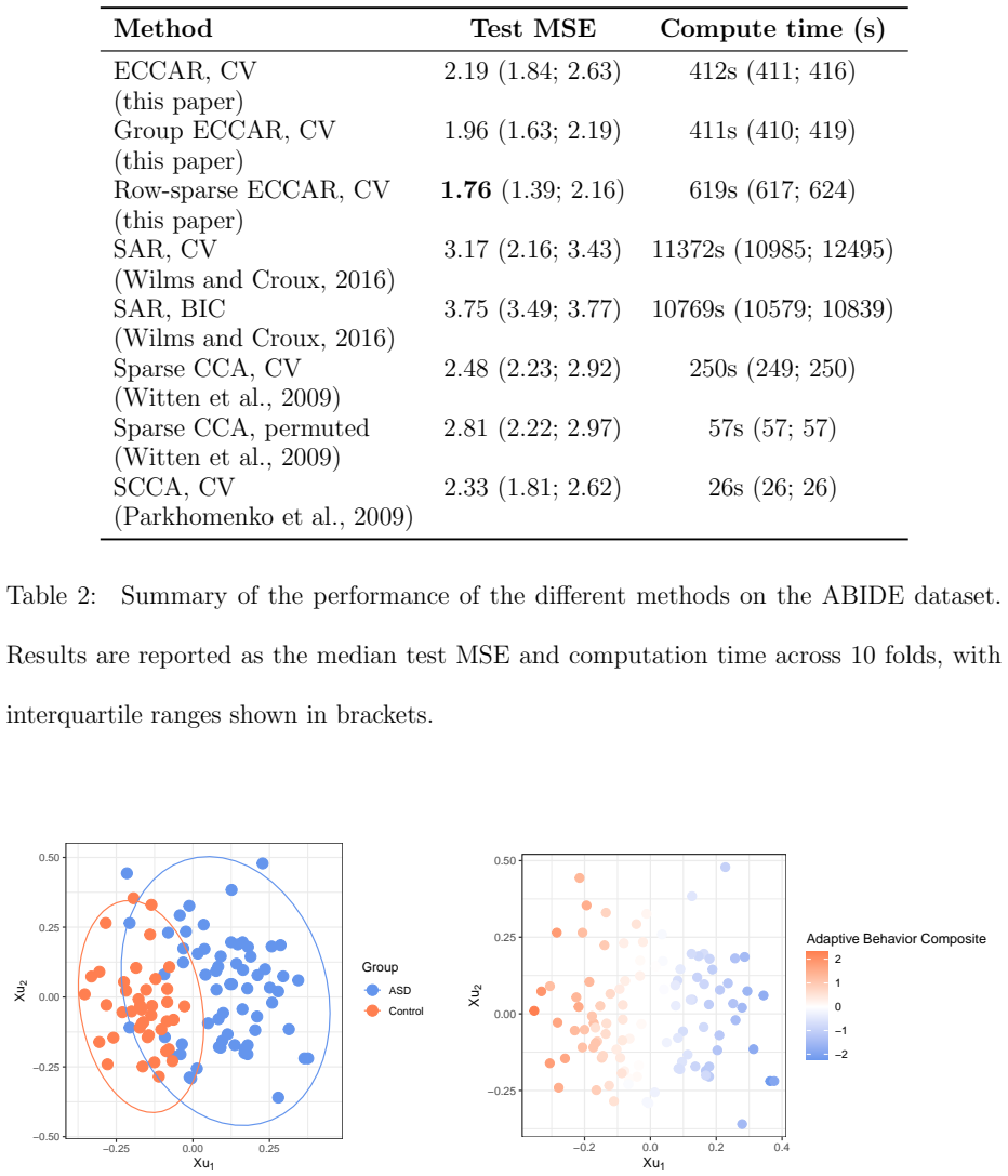
Summary. The paper proposes ECCAR, a sparse canonical correlation analysis method that estimates the population matrix B* = U*Λ*V*^T by solving the convex Lasso-type problem in Eq. (8), then extracts canonical directions through a rank-r SVD and normalization (Algorithm 1). The main theoretical results are Theorem 3.1, giving a Frobenius-norm error bound of order sqrt(s_u s_v log(p+q)/n) for the estimate of B*; Theorem 3.2, giving a direction-estimation error bound of order (1/λ_r^2) sqrt(s_u s_v log(p+q)/n); and Theorem 3.3 with Corollary 3.3.1, providing support-recovery guarantees under an irrepresentable-type condition. The paper also reports extensive simulations and applications to AUD genetics, ABIDE neuroimaging, and LLM embedding interpretability, and it makes an R package available.
Significance. If the central consistency results are correct, ECCAR is a useful addition to the sparse CCA toolbox: it avoids Fantope projections, does not require sample splitting, and the reported simulations suggest substantial computational gains over existing theory-based methods. The proof of Theorem 3.1 follows standard Lasso techniques and is plausible. However, the paper's advertised support-recovery and 'sparsistency' contribution is materially stronger than what the theorems prove, and the proof of the high-probability support-inclusion corollary contains a gap. The direction-consistency rate in Theorem 3.2 is also acknowledged to be slower than minimax rates, so the significance rests mainly on computation and practical performance rather than on optimal statistical efficiency.
major comments (3)
- [§1 Contribution (2); §3.2; §6] The paper advertises support recovery and 'sparsistency', but Theorem 3.3 and Corollary 3.3.1 only prove supp(hat B) ⊆ S_u × S_v, i.e., absence of false positives. They do not establish supp(hat B) = S_u × S_v, nor do they guarantee that all true support variables are recovered. The paragraph after Corollary 3.3.1 similarly only gives inclusion for hat U and hat V. Since Section 6 defines 'sparsistent' as coming with provable guarantees on identified variables, the conclusion that ECCAR is 'the first estimator ... that provably meets all three criteria' overstates the result. Please either prove exact support recovery under an additional signal-strength (beta-min) condition or reframe the contribution as false-positive control and support inclusion.
- [Appendix F.1.3, proof of Corollary 3.3.1] The high-probability version of the irrepresentable condition is not established by the cited lemmas. The proof asserts, immediately after invoking Lemma D.3, that ||(hat Σ_X)_{S_u^c S_u}||_{2,∞} ≤ ||(Σ_X)_{S_u^c S_u}||_{2,∞} + a√s_u √(log(p+q)/n) (and similarly for Y). Lemma D.3 controls the entrywise infinity norm of hat Σ_XY - hat Σ_X B* hat Σ_Y, and Lemma D.4 controls sparse eigenvalues; neither directly gives the stated 2,∞ block-norm deviation. A separate concentration argument for block row norms is needed. As written, the proof of Corollary 3.3.1 is incomplete, which is load-bearing because the corollary is the main support-recovery guarantee.
- [Eq. (12) and §3.2] Even if the proof gap is repaired, the support guarantee is conditional on the population irrepresentable condition in Eq. (12), which is not checkable from the data and fails when in-support and out-of-support variables are highly correlated. The paper does not provide a data-dependent verification procedure or a fallback guarantee for that regime. Because the support-recovery claim is one of the three advertised contributions and is used in the conclusion to claim that ECCAR 'provably meets all three criteria', this limitation should be stated explicitly in Section 3.2 and the conclusion, and the claims should be softened accordingly.
minor comments (4)
- [Theorem 3.2 and Appendix F.1.4] There is a notation mismatch: the main-text Theorem 3.2 uses λ_r^{*2} in the sample-size condition, while the appendix statement of the same theorem uses ρ_r^{*2}. Also, within the proof of Theorem 3.2 in Appendix F.1.4, the text says 'Following the same logic as in the proof of Theorem 3.2', which appears to be a self-reference; this should likely refer to Theorem 3.1.
- [Appendix F.1.3, proof of Corollary 3.3.1] The concentration display for the sample covariance blocks contains a likely typo: the sequence lists σmin(bΣY) twice where one instance should presumably be σmax(bΣY), since the intended result is a two-sided bound on both restricted eigenvalues.
- [Table 3] The row for Gao and Ma (2023) contains 'r(su+sv)rlog(p+q)' with a duplicated 'r'; the displayed rate should be cleaned up for readability.
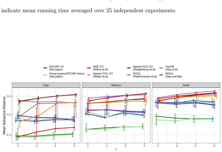
- [§4, Figure 1] The main text refers to the 'sin Θ distance between the stacked (U*,V*) and the estimates', but no formal definition of this distance is given; please define it explicitly for reproducibility.
Circularity Check
No significant circularity: ECCAR's estimator and error bounds are derived from the stated canonical-pair model with independent external lemmas; the only self-citation is a conceptual pointer, not a load-bearing result.
full rationale
The paper's central chain is self-contained and non-circular. The estimator of B* = U*Lambda*V*^T is defined by the convex problem in Eq. 8, and Theorem 2.1 derives its population limit (and the low-dimensional consistency) directly from the KKT condition bB = bSigma_X^{-1} bSigma_XY bSigma_Y^{-1} and the canonical-pair reparametrization Sigma_XY = Sigma_X U* Lambda* V*^T Sigma_Y. No fitted parameter is relabeled as a prediction: rho is a tuning parameter chosen by theory or cross-validation, and the reported test metrics are out-of-fold. The high-dimensional consistency proofs (Theorems 3.1 and 3.2) rely on external matrix-perturbation and concentration results (Yu et al. 2015, Klopp et al. 2021) and on lemmas from Gao et al. 2017, all independent of the authors' own prior work. The support-recovery result (Theorem 3.3/Corollary 3.3.1) is a standard irrepresentable-type sufficient condition and is not an input renamed as an output; it guarantees only supp(hat B) subset of Su x Sv, which is weaker than the 'sparsistent' language in Section 6 but is an over-claim about the theorem's content, not a circularity. The paper cites Donnat and Tuzhilina (2024) (two of the present authors) for the reduced-rank-regression viewpoint, but the current formulation is explicitly presented as distinct, and its properties are proved afresh rather than imported from that citation. No circular step satisfies the requirement of being exhibited as Eq. X = Eq. Y by construction or as a fitted parameter renamed as a prediction.
Assumptions & free parameters
free parameters (3)
- rho (regularization parameter) =
chosen by cross-validation or theoretical formula
- r (number of canonical directions) =
2 for AUD and ABIDE, 4/10 for LLM, 5 for Nutrimouse
- group structure G =
36 network interaction groups for ABIDE; 5x5 blocks in simulations
assumptions (4)
- domain assumption Data are i.i.d. Gaussian with covariance satisfying the canonical pair model (Eq. 3).
- domain assumption Canonical directions are row-sparse: |supp(U*)| ≤ s_u and |supp(V*)| ≤ s_v.
- domain assumption Covariances are well-conditioned: 1/M ≤ σ_min(Σ_X) ∧ σ_min(Σ_Y) and σ_max(Σ_X) ∨ σ_max(Σ_Y) ≤ M.
- ad hoc to paper Irrepresentable condition (Eq. 12) holds: cross-covariance between support and outside-support is sufficiently small.
Cite this review
Pith. "Pith review of Efficient Canonical Correlation Analysis with Sparsity." pith.science (2026). https://pith.science/paper/5HZU36E3
@misc{pith2026250711160,
  author       = {Pith},
  title        = {Pith review of: Efficient Canonical Correlation Analysis with Sparsity},
  year         = {2026},
  howpublished = {\url{https://pith.science/paper/5HZU36E3}},
  note         = {Machine review of arXiv:2507.11160}
}
read the original abstract
In high-dimensional settings, Canonical Correlation Analysis (CCA) often fails, and existing sparse methods force an untenable choice between computational speed and statistical rigor. This work introduces a fast and provably consistent sparse CCA algorithm (ECCAR) that resolves this trade-off. We formulate CCA as a high-dimensional reduced-rank regression problem, which allows us to derive consistent estimators with high-probability error bounds without relying on computationally expensive techniques like Fantope projections. The resulting algorithm is scalable, projection-free, and significantly faster than its competitors. We validate our method through extensive simulations and demonstrate its power to uncover reliable and interpretable associations in two complex biological datasets, as well as in an ML interpretability task. Our work makes sparse CCA a practical and trustworthy tool for large-scale multimodal data analysis. A companion R package has been made available.
Figures


Figures from the paper (20 more)






Reference graph
Works this paper leans on
-
[1]
Andrew, G., Arora, R., Bilmes, J., and Livescu, K. (2013). Deep canonical correlation analysis. In International conference on machine learning , pages 1247--1255. PMLR
work page 2013
-
[2]
B., Tustison, N., Song, G., et al
Avants, B. B., Tustison, N., Song, G., et al. (2009). Advanced normalization tools (ANTS) . Insight j , 2(365):1--35
work page 2009
-
[3]
Behzadi, Y., Restom, K., Liau, J., and Liu, T. T. (2007). A component based noise correction method (compcor) for bold and perfusion based fmri. Neuroimage , 37(1):90--101
work page 2007
-
[4]
Boyd, S., Parikh, N., Chu, E., Peleato, B., and Eckstein, J. (2011). Distributed optimization and statistical learning via the alternating direction method of multipliers. Foundations and Trends in Machine Learning , 3:1--122
work page 2011
-
[5]
Chen, M., Gao, C., Ren, Z., and Zhou, H. H. (2013). Sparse CCA via precision adjusted iterative thresholding . arXiv preprint arXiv:1311.6186
work page Pith review arXiv 2013
-
[6]
S., Yan, C., Li, Q., Lurie, D., Vogelstein, J., Burns, R., et al
Craddock, C., Sikka, S., Cheung, B., Khanuja, R., Ghosh, S. S., Yan, C., Li, Q., Lurie, D., Vogelstein, J., Burns, R., et al. (2013). Towards automated analysis of connectomes: The configurable pipeline for the analysis of connectomes (c-pac). Front Neuroinform , 42(10.3389)
work page 2013
-
[7]
S., S \'e gonne, F., Fischl, B., Quinn, B
Desikan, R. S., S \'e gonne, F., Fischl, B., Quinn, B. T., Dickerson, B. C., Blacker, D., Buckner, R. L., Dale, A. M., Maguire, R. P., Hyman, B. T., et al. (2006). An automated labeling system for subdividing the human cerebral cortex on mri scans into gyral based regions of interest. Neuroimage , 31(3):968--980
work page 2006
-
[8]
Di Martino, A., Yan, C.-G., Li, Q., Denio, E., Castellanos, F. X., Alaerts, K., Anderson, J. S., Assaf, M., Bookheimer, S. Y., Dapretto, M., et al. (2014). The autism brain imaging data exchange: towards a large-scale evaluation of the intrinsic brain architecture in autism. Molecular psychiatry , 19(6):659--667
work page 2014
Show all 52 references
-
[9]
and Tuzhilina, E
Donnat, C. and Tuzhilina, E. (2024). Canonical correlation analysis as reduced rank regression in high dimensions. arXiv preprint arXiv:2405.19539
2024 arXiv
-
[10]
Dos Santos, S. F. and Brandi, H. S. (2014). A canonical correlation analysis of the relationship between sustainability and competitiveness. Clean Technologies and Environmental Policy , 16:1735--1746
2014
-
[11]
and Konold, T
Fan, X. and Konold, T. R. (2018). Canonical correlation analysis. In The reviewer’s guide to quantitative methods in the social sciences , pages 29--41. Routledge
2018
-
[12]
Gao, C., Ma, Z., Ren, Z., and Zhou, H. H. (2015). Minimax estimation in sparse canonical correlation analysis. The Annals of Statistics , 43(5):2168--2197
2015
-
[13]
Gao, C., Ma, Z., and Zhou, H. H. (2017). Sparse CCA: Adaptive estimation and computational barriers . The Annals of Statistics , 45(5):2074--2101
2017
-
[14]
and Ma, Z
Gao, S. and Ma, Z. (2023). Sparse gca and thresholded gradient descent. Journal of Machine Learning Research , 24(135):1--61
2023
-
[15]
P., Kusumo, H., Zhang, H., Guidotti, A., and Pandey, S
Gavin, D. P., Kusumo, H., Zhang, H., Guidotti, A., and Pandey, S. C. (2016). Role of growth arrest and dna damage-inducible, beta in alcohol-drinking behaviors. Alcoholism: Clinical and Experimental Research , 40(2):263--272
2016
-
[16]
M., Buchsbaum, M
Haznedar, M. M., Buchsbaum, M. S., Wei, T.-C., Hof, P. R., Cartwright, C., Bienstock, C. A., and Hollander, E. (2000). Limbic Circuitry in Patients With Autism Spectrum Disorders Studied With Positron Emission Tomography and Magnetic Resonance Imaging . American Journal of Psy...
2000
-
[17]
L., Howell, A., Rosand, B., Anticevic, A., Sotiropoulos, S
Helmer, M., Warrington, S., Mohammadi-Nejad, A.-R., Ji, J. L., Howell, A., Rosand, B., Anticevic, A., Sotiropoulos, S. N., and Murray, J. D. (2024). On the stability of canonical correlation analysis and partial least squares with application to brain-behavior associations. Co...
2024
-
[18]
Hotelling, H. (1936). Relations between two sets of variates. In Biometrika, 28 , pages 321--377. Springer
1936
-
[19]
Hu, R., Dai, Y., Jia, P., and Zhao, Z. (2018). ANCO-GeneDB : Annotations and comprehensive analysis of candidate genes for alcohol, nicotine, cocaine, and opioid dependence. https://bioinfo.uth.edu/ancogenedb/views/meDNA.php. Database; DOI:10.1093/database/bay121
2018 doi
-
[20]
B., Gerszten, R
Jiang, M.-Z., Aguet, F., Ardlie, K., Chen, J., Cornell, E., Cruz, D., Durda, P., Gabriel, S. B., Gerszten, R. E., Guo, X., et al. (2023). Canonical correlation analysis for multi-omics: Application to cross-cohort analysis. PLoS genetics , 19(5):e1010517
2023
-
[21]
Jordan, C. (1875). Essai sur la g \'e om \'e trie \`a n dimensions. Bulletin de la Soci \'e t \'e math \'e matique de France , 3:103--174
-
[22]
Klopp, O., Panov, M., Sigalla, S., and Tsybakov, A. (2021). Assigning topics to documents by successive projections. arXiv preprint arXiv:2107.03684
2021 arXiv
-
[23]
G., Robert-Grani \'e , C., and Besse, P
L \^e Cao, K.-A., Martin, P. G., Robert-Grani \'e , C., and Besse, P. (2009). Sparse canonical methods for biological data integration: application to a cross-platform study. BMC bioinformatics , 10:1--17
2009
-
[24]
D., Deng, H.-W., and Wang, Y.-P
Lin, D., Zhang, J., Li, J., Calhoun, V. D., Deng, H.-W., and Wang, Y.-P. (2013). Group sparse canonical correlation analysis for genomic data integration. BMC bioinformatics , 14(1):1--16
2013
-
[25]
E., Madsen, K
Lund, T. E., Madsen, K. H., Sidaros, K., Luo, W.-L., and Nichols, T. E. (2006). Non-white noise in fmri: does modelling have an impact? Neuroimage , 29(1):54--66
2006
-
[26]
K., and Chen, K
Luo, C., Liu, J., Dey, D. K., and Chen, K. (2016). Canonical variate regression. Biostatistics , 17(3):468--483
2016
-
[27]
G., Guillou, H., Lasserre, F., D \'e jean, S., Lan, A., Pascussi, J.-M., SanCristobal, M., Legrand, P., Besse, P., and Pineau, T
Martin, P. G., Guillou, H., Lasserre, F., D \'e jean, S., Lan, A., Pascussi, J.-M., SanCristobal, M., Legrand, P., Besse, P., and Pineau, T. (2007). Novel aspects of ppar -mediated regulation of lipid and xenobiotic metabolism revealed through a nutrigenomic study. Hepatology ...
2007
-
[28]
Mazuruse, P. (2014). Canonical correlation analysis: Macroeconomic variables versus stock returns. Journal of Financial Economic Policy , 6(2):179--196
2014
-
[29]
N., McBride, W
McClintick, J. N., McBride, W. J., Bell, R. L., Ding, Z.-M., Liu, Y., Xuei, X., and Edenberg, H. J. (2018). Gene expression changes in the ventral hippocampus and medial prefrontal cortex of adolescent alcohol-preferring (p) rats following binge-like alcohol drinking. Alcohol ...
2018
-
[30]
McIntosh, A. R. (2021). Comparison of canonical correlation and partial least squares analyses of simulated and empirical data. arXiv preprint arXiv:2107.06867
2021 arXiv
-
[31]
Morcos, A., Raghu, M., and Bengio, S. (2018). Insights on representational similarity in neural networks with canonical correlation. Advances in neural information processing systems , 31
2018
-
[32]
L., McIntosh, A
Nakua, H., Yu, J.-C., Abdi, H., Hawco, C., Voineskos, A., Hill, S., Lai, M.-C., Wheeler, A. L., McIntosh, A. R., and Ameis, S. H. (2024). Comparing the stability and reproducibility of brain-behavior relationships found using canonical correlation analysis and partial least sq...
2024
-
[33]
Parkhomenko, E., Tritchler, D., and Beyene, J. (2009). Sparse canonical correlation analysis with application to genomic data integration. Statistical applications in genetics and molecular biology , 8(1)
2009
-
[34]
Raghu, M., Gilmer, J., Yosinski, J., and Sohl-Dickstein, J. (2017). Svcca: Singular vector canonical correlation analysis for deep learning dynamics and interpretability. Advances in neural information processing systems , 30
2017
-
[35]
M., Masamunt, M
Revilla, L., Mayorgas, A., Corraliza, A. M., Masamunt, M. C., Metwaly, A., Haller, D., Trist \'a n, E., Carrasco, A., Esteve, M., Pan \'e s, J., et al. (2021). Multi-omic modelling of inflammatory bowel disease with regularized canonical correlation analysis. Plos one , 16(2):e0246367
2021
-
[36]
Rodosthenous, T., Shahrezaei, V., and Evangelou, M. (2020). Integrating multi-omics data through sparse canonical correlation analysis for the prediction of complex traits: a comparison study. Bioinformatics , 36(17):4616--4625
2020
-
[37]
Rohart, F., Gautier, B., Singh, A., and L \^e Cao, K.-A. (2017). mixomics: An r package for ‘omics feature selection and multiple data integration. PLoS computational biology , 13(11):e1005752
2017
-
[38]
E., Li, S., and Long, Q
Safo, S. E., Li, S., and Long, Q. (2018). Integrative analysis of transcriptomic and metabolomic data via sparse canonical correlation analysis with incorporation of biological information. Biometrics , 74(1):300--312
2018
-
[39]
S., Cicchetti, D
Sparrow, S. S., Cicchetti, D. V., and Balla, D. A. (2005). Vineland Adaptive Behavior Scales, Second Edition (Vineland-II): Survey Forms Manual . AGS Publishing
2005
-
[40]
Stewart, G. (1969). On the continuity of the generalized inverse. SIAM Journal on Applied Mathematics , 17(1):33--45
1969
-
[41]
Thorndike, R. M. (2000). Canonical correlation analysis. In Handbook of applied multivariate statistics and mathematical modeling , pages 237--263. Elsevier
2000
-
[42]
Tibshirani, R. (1996). Regression shrinkage and selection via the lasso. Journal of the Royal Statistical Society Series B: Statistical Methodology , 58(1):267--288
1996
-
[43]
and Zwinderman, A
Waaijenborg, S. and Zwinderman, A. H. (2009). Sparse canonical correlation analysis for identifying, connecting and completing gene-expression networks. BMC Bioinformatics , 10
2009
-
[44]
and Croux, C
Wilms, I. and Croux, C. (2015). Sparse canonical correlation analysis from a predictive point of view. Biometrical Journal , 57(5):834--851
2015
-
[45]
and Croux, C
Wilms, I. and Croux, C. (2016). Robust sparse canonical correlation analysis. BMC Systems Biology , 10(72)
2016
-
[46]
M., Tibshirani, R., and Hastie, T
Witten, D. M., Tibshirani, R., and Hastie, T. (2009). A penalized matrix decomposition, with applications to sparse principal components and canonical correlation analysis. Biostatistics , 10(3):515--534
2009
-
[47]
Witten, D. M. and Tibshirani, R. J. (2009). Extensions of sparse canonical correlation analysis with applications to genomic data. Statistical applications in genetics and molecular biology , 8(1)
2009
-
[48]
T., Krienen, F
Yeo, B. T., Krienen, F. M., Sepulcre, J., Sabuncu, M. R., Lashkari, D., Hollinshead, M., Roffman, J. L., Smoller, J. W., Z \"o llei, L., Polimeni, J. R., et al. (2011). The organization of the human cerebral cortex estimated by intrinsic functional connectivity. Journal of neu...
2011
-
[49]
Yu, Y., Wang, T., and Samworth, R. J. (2015). A useful variant of the Davis--Kahan theorem for statisticians . Biometrika , 102(2):315--323
2015
-
[50]
Zeng, L.-P., Qin, Y.-Q., Lu, X.-M., Feng, Z.-B., and Fang, X.-L. (2023). Identify gadd45g as a potential target of 4-methoxydalbergione in treatment of liver cancer: bioinformatics analysis and in vivo experiment. World Journal of Surgical Oncology , 21(1):324
2023
-
[51]
Zhang, H., Wang, F., Xu, H., Liu, Y., Liu, J., Zhao, H., and Gelernter, J. (2014). Differentially co-expressed genes in postmortem prefrontal cortex of individuals with alcohol use disorders: influence on alcohol metabolism-related pathways. Human genetics , 133:1383--1394
2014
-
[52]
Zhang, Y., Zhan, C., Chen, G., and Sun, J. (2018). Label-free quantitative proteomics and bioinformatics analyses of alcoholic liver disease in a chronic and binge mouse model. Molecular Medicine Reports , 18(2):2079--2087
2018
Reviewed August 6, 2026 · model on record in the stance chip above.
Discussion (0). Continue with ORCID to comment.