Automatic reproducing kernel and regularization for learning convolution kernels

Fei Lu; Haibo Li

REVIEW 2 major objections 6 minor 50 references

Automatic reproducing kernel and regularization for learning convolution kernels

T0 review · 2 major / 6 minor · reviewed 2026-08-06 · deepseek-v4-flash

Challenge this review Re-run · record.json Download PDF Read on arXiv ↗ Review JSON

Pith's one-line read Convolution kernels can be learned from discrete noisy data without manual reproducing-kernel selection, because the data and forward operator themselves induce an automatic RKHS in which all estimators reduce to finite matrix problems.

desk verdict The central representer theorem and the CG/GKB machinery are sound and genuinely useful, but the discrete-data transition and the "no hyperparameter tuning" claim need honest qualification before the practical conclusions can be taken at face value. read the letter →

arxiv 2507.11944 v1 pith:LO244FNH submitted 2025-07-16 math.NA cs.NA

Haibo Li , Fei Lu This is my paper · ORCID

classification math.NAcs.NA MSC 65J2245Q0562G08

keywords automaticreproducingkernelconvolutionlearningdata-adaptiveRKHSdeconvolutioninverseproblemfinite-dimensionalrepresentertheoremTikhonovregularizationGolub-Kahanbidiagonalizationoperator

verification ladder T0 review T1 audit T2 compute T3 formal

The pith

A machine-rendered reading of the paper's core claim, the machinery that carries it, and where it could break.

The reading

This paper claims that for learning a convolution kernel from discrete, noisy input–output data, the data and the forward operator themselves determine a data-adaptive reproducing kernel Hilbert space (DA-RKHS), removing the usual need to pick a Gaussian or Matérn kernel by hand. The central result is a finite-dimensional representer theorem: even though the minimization runs over an infinite-dimensional space, the minimal-norm least-squares, Tikhonov, and conjugate-gradient estimators all lie in the span of finitely many automatic basis functions built from the data. Learning the kernel therefore collapses to a finite matrix problem whose solution is given by the pseudoinverse formulas $\hat{c}=\Sigma^{+}f$ or $\hat{c}_\lambda=(\Sigma^2+n_0J\lambda\Sigma)^{+}\Sigma f$. If this is right, the main practical bottleneck of kernel methods for deconvolution-type inverse problems—kernel and hyperparameter selection—disappears. Experiments on integral, nonlocal, and aggregation operators show the automatic regularization consistently beating ridge regression and Gaussian-process methods with preselected kernels.

What carries the argument

The central object is the automatic reproducing kernel $G(s,s')=\bar G(s,s')/(\dot\rho(s)\dot\rho(s'))\mathbf{1}_{\dot\rho(s)\dot\rho(s')>0}$, built from the empirical normal operator $\bar G(s,s')$ and the exploration measure $\dot\rho(s)$; its RKHS is $H_G=L_G^{1/2}(L^2_\rho)$ with closure $H=N(L_G)^\perp$, the identifiable subspace. The finite representer theorem is the load-bearing mechanism: the functions $\xi_{kj}(s)=\int_S G(s,s')g[u_k](x_j,s')\,ds'$ are representers of the bounded linear functionals $\varphi\mapsto R_\varphi[u_k](x_j)$ on $H_G$, so the variational loss becomes $\frac{1}{n_0J}\|\Sigma c-f\|_2^2$ with penalty $\lambda c^T\Sigma c$ in coefficient space. The pseudoinverse formulas $\hat{c}=\Sigma^{+}f$ and $\hat{c}_\lambda=(\Sigma^2+n_0J\lambda\Sigma)^{+}\Sigma f$ are the resulting finite-dimensional implementations, and the Golub–Kahan bidiagonalization of $\tilde{T}:x\mapsto\Sigma x$ on $N(\Sigma)^\perp$ yields the iterative and hybrid solvers.

What would settle it

For a fixed operator and data, compute the Gram matrix $\Sigma$ by high-accuracy quadrature and compare the coefficient-form estimator $\hat{c}_\lambda^T\xi$ against a direct discretized solution of the infinite-dimensional Tikhonov problem (2.6) on a very fine grid of $S$; if the two do not converge to the same function as the grid refines, the finite representer theorem would be false. Alternatively, test with a true kernel supported where $\dot\rho=0$ and noise-free data: the paper predicts the estimator is identically zero there, and any data-driven method that recovers the kernel in that region would require a hypothesis space larger than $H_G$.

Watch

Extended reading notes

Core claim

The paper establishes that for estimating the kernel $\varphi$ in $R_\varphi[u](x)=\int_S \varphi(s)g[u](x,s)\,ds$ from finite noisy pairs, the variational estimator over the infinite-dimensional RKHS $H_G$ of the automatic kernel $G$ has an explicit finite-dimensional representation. The automatic kernel is $G(s,s')=\bar G(s,s')/(\dot\rho(s)\dot\rho(s'))\mathbf{1}_{\{\dot\rho(s)\dot\rho(s')>0\}}$ with $\bar G(s,s')=\frac{1}{n_0}\sum_k\int_X g[u_k](x,s)g[u_k](x,s')\,\nu(dx)$, weighted by the exploration measure $\dot\rho(s)=\frac{1}{n_0Z}\sum_{k,j}|g[u_k](x_j,s)|\Delta x$. Theorem 2.5 constructs automatic basis functions $\xi_{kj}(s)=\int_S G(s,s')g[u_k](x_j,s')\,ds'$ that represent the linear functionals $R_\varphi[u_k](x_j)$ on $H_G$; the Gram matrix $\Sigma=(\langle\xi_{kj},\xi_{k'j'}\rangle_{H_G})$ then carries the whole optimization, with coefficients $\hat{c}=\Sigma^{+}f$ and $\hat{c}_\lambda=(\Sigma^2+n_0J\lambda\Sigma)^{+}\Sigma f$. These formulas project out the null-space component of the noise, avoid the small-noise blow-up of plain ridge regression when $\Sigma$ is singular, and reduce to the ridge estimator when $\Sigma$ is invertible. The paper adds conjugate-gradient/Golub–Kahan iterative and hybrid algorithms and piecewise-constant discrete-data approximations, and demonstrates convergence and speed advantages in three examples.

Load-bearing premise

The data must actually explore every direction of the kernel's domain that one wants to recover: wherever the exploration measure $\dot\rho(s)$ is zero, the automatic kernel is set to zero and the estimator cannot detect kernel components living there.

Editorial extensions

If this is right

No manual kernel or bandwidth selection is needed: the data and forward operator supply both the hypothesis space and the regularizer, so Tikhonov and iterative estimators are computed directly from the Gram matrix $\Sigma$.
When $\Sigma$ is singular, the Tikhonov estimator $(\Sigma^2+n_0J\lambda\Sigma)^{+}\Sigma f$ stays in $N(\Sigma)^\perp$ and avoids contamination by $P_{N(\Sigma)}f$, whereas ridge regression $(\Sigma+n_0J\lambda I)^{-1}f$ can blow up as noise vanishes.
The conjugate-gradient iterates on $H_G$ correspond to coefficient-space Krylov subspaces $\mathcal{K}_l=\mathrm{span}\{\Sigma^i\Sigma^{+}f\}_{i=1}^l$, so the seemingly infinite-dimensional regularization is exactly a finite-dimensional matrix problem at every iteration.
The methods are mesh-free in the sense that the automatic basis functions $\xi_{kj}$ are used directly when the functions $g[u_k](x_j,\cdot)$ are known analytically, and the piecewise-constant approximation in Section 3 makes them computable from raw discrete data.
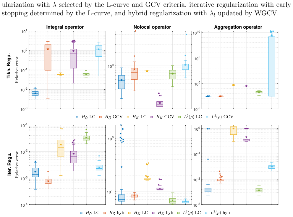
Experiments on integral, nonlocal, and aggregation operators indicate the $H_G$-norm estimator converges as noise decreases and outperforms Gaussian-kernel and $L^2_\rho$ regularizers, with the hybrid method the most stable.

Reading between the lines

Editorial extensions of the paper, not claims the author makes directly.

The finite representer theorem suggests the effective dimension of the deconvolution problem is at most $n_0J$ (and no larger than the numerical rank of $\Sigma$), so one would expect minimax rates governed by the eigenvalue decay of $L_G$; the paper does not state such rates.
The exploration measure $\dot\rho$ acts as an automatic adaptive quadrature weight: a practical consequence, left implicit in the paper, is that one can design input data $u_k$ to push $\dot\rho$ toward regions of $S$ where kernel resolution is needed.
Because the learned kernels are exactly the convolution kernels used in nonlocal and neural-operator layers, the automatic basis could serve as a feature map for operator learning, though the paper does not explore this connection.
A sharp test of the method's limits would be to apply it to a real peridynamics or particle-system dataset where the true kernel is not known to lie close to the identifiable space $H$; the numerical demonstrations use test kernels close to $H$, leaving that regime untested.

Share X Bluesky LinkedIn Reddit HN

Editorial analysis

A structured set of objections, weighed in public.

Desk editor's note, referee report, and a circularity audit.

Desk Editor's Note

read the letter

Short version: this paper is worth a serious referee, and the central theorem survives contact. The genuinely new content is Theorem 2.5, the automatic-basis representer result, plus the coefficient-space CG/GKB equivalences (Theorems 2.8-2.9) and the practical discrete-data formulation. I checked the core algebra; (2.9) and (2.10) are right, and the Tikhonov form (Sigma^2 + n0 J lambda Sigma)^+ Sigma f correctly avoids the null-space contamination that plain ridge would suffer. The GKB derivations also hang together. That is real progress: learning a convolution kernel in a linear-in-kernel operator becomes a finite matrix problem with no manual choice of reproducing kernel.

The soft spots are mostly about claims versus proof. The abstract says "obviating manual kernel selection," but lambda, the stopping iteration, lmax, the rank threshold, and the discrepancy constant tau are still selected; only the kernel itself is automatic. The GP baseline uses one fixed bandwidth sigma0 = 0.1, so "consistently outperforms GP" is a statement about one untuned baseline, not about the method class. Section 5 also says the true kernels are chosen close to the identifiable space H; that is the favorable regime, and the paper owns it.

The more serious gap is the discrete transition. Theorem 2.5 is proved for semi-continuum data {g[u_k](x_j, .)}. In Section 3, the functions are replaced by piecewise constants, and the discrete basis functions are not shown to lie in H_G. So the computed estimator (3.4) is not proved to minimize (2.6) over H_G, and there is no discretization error bound. The "mesh-free" claim is stronger than what is proved. This does not sink the paper—the numerical experiments are reproducible and the algebra on the discrete side is sensible—but it means the practical claim rests on numerics for now.

Who is this for: anyone doing kernel learning for integral, nonlocal, or aggregation operators, or data-driven nonlocal PDE identification. The paper deserves a serious referee and probably a round of revision. I would send it out, asking for a discretization error estimate or at least an honest statement that the discrete estimator is a heuristic approximation of the Theorem 2.5 minimizer, plus a toned-down abstract.

Referee Report

2 major / 6 minor

Summary. The paper proposes a data-adaptive reproducing kernel Hilbert space (DA-RKHS) for learning convolution kernels in linear-in-kernel operators from input-output data. An exploration measure and an automatic kernel are constructed from the input features and the forward operator, and a finite-dimensional representer theorem (Theorem 2.5) is proved for semi-continuum observations, giving coefficient formulas for the minimal-norm least-squares and Tikhonov estimators. Conjugate-gradient and Golub-Kahan iterative/hybrid algorithms are developed, followed by a discrete approximation in Section 3 and numerical experiments on integral, nonlocal, and aggregation operators showing that the proposed HG-norm regularization often outperforms Gaussian-kernel and L2-rho baselines.

Significance. If the main claims hold, the paper offers a useful and practically motivated idea: replacing manual kernel selection by a kernel constructed from the data and forward operator, and reducing an infinite-dimensional variational problem to a finite matrix problem for several estimators. The core identities in Theorems 2.5, 2.8, and 2.9 are internally consistent, the pseudoinverse-based Tikhonov formula correctly blocks null-space noise, and the numerical study is extensive with public code. The significance is reduced, however, by the gap between the idealized semi-continuum setting of the representer theorem and the genuinely discrete data setting of the algorithms and experiments, which is not accompanied by error bounds.

major comments (2)

[Section 3, Eqs. (3.1)-(3.4)] Theorem 2.5 is proved under the assumption that the functions s -> g[u_k](x_j,s) are known on the whole interval S (semi-continuum data). In the actual discrete setting of (1.2), only point values are available, and Section 3 replaces these functions by piecewise constants (3.1), producing discrete basis functions that are not, in general, elements of the infinite-dimensional space H_G. The computed estimator (3.4) is therefore not shown to be the minimizer of the variational problem (2.6) over H_G, and no discretization or quadrature error bound is supplied. Consequently, the advertised reduction to a finite matrix problem, and the 'mesh-free' and 'automatic' claims in the abstract and conclusion, are stronger than what is rigorously proved. The authors should either provide a discretization error analysis (e.g., convergence of the discrete estimator to the H_G-minimizer as the s-mesh and x-mesh sizes tend to zero under suitable regularity conditions) or explicitly restate the practical claims as heuristic for the discrete-data setting.
[Section 5, 'Numerical settings'] The manuscript states that the true kernels are deliberately chosen 'close to the identifiable spaces H' for each example, making accurate estimation possible. This is an explicit limitation: the experiments live in the favorable regime where the exploration measure covers the support of the kernel and the kernel has no significant component in N(L_G). The abstract and conclusion do not carry this caveat, so a reader may overestimate the method's guarantees. Please state this identifiability restriction in the abstract or conclusion, and ideally add at least one experiment in which the kernel's support extends into a region where the exploration measure vanishes, to demonstrate the behavior of the estimator in that regime.

minor comments (6)

[Section 2.3, Eq. (2.9)] The notation 'Σ:' for the pseudoinverse is used without an explicit definition at first occurrence; please define it clearly (e.g., 'Σ: denotes the Moore-Penrose pseudoinverse').
[Appendix A, first line] The proof heading reads 'Proof of Theorem 2.4', but the statement in the main text is Lemma 2.4; please correct the label.
[Section 3, Table 1 and Eq. (3.2)] Several displayed formulas contain typographical artifacts such as 'p9ρDpsq' and '9ρ_Discrete'; these should be cleaned up.
[Section 5, Figure 1 caption] The caption contains the typo 'Nolocal operator'; it should read 'Nonlocal operator'.
[Algorithm 2, line 4] The initialization divides by β1 = ||P_{N(Σ_D)^⊥} f||_2; if this quantity is zero (i.e., f is orthogonal to the range of Σ_D), the algorithm divides by zero. This degenerate case should be addressed or excluded explicitly.
[Abstract and Section 5] The abstract refers to 'Gaussian process methods' as baselines, but the experiments compare against Tikhonov and iterative regularization using a Gaussian kernel norm, which is not the same as Gaussian process regression; please adjust the wording for accuracy.

Circularity Check

0 steps flagged · score 0.0 of 10

No significant circularity: the finite-dimensional representer theorem is proved from the paper's definitions and the estimator formulas are derived algebraically; self-citations are contextual rather than load-bearing.

full rationale

The paper's central claim, Theorem 2.5, is not circular. The automatic kernel G in (2.3) and the basis functions ξ_kj in (2.7) are constructed directly from the input features {g[u_k](x_j,·)} and the forward operator, never from the output labels f. The representer theorem is then proved from Lemma 2.4(c) and the definition of the RKHS inner product: the identity <ξ_kj, φ>_{H_G} = R_φ[u_k](x_j) follows algebraically, and the loss functions E_D and E_λ are exactly rewritten as finite-dimensional problems in Σ and f. Formulas (2.9) and (2.10) are derived from those algebraic reductions, not imposed by a fitted parameter or by a prior result. The self-citations [8], [31], [36], [37], and [50] provide background, small-noise analysis, and convergence rates, but none of them supplies the finite-dimensional representer property; the proof in Appendix A is self-contained. Two limitations should be noted but neither is circular. First, Section 3 approximates the continuum functions g[u_k](x_j,·) by piecewise constants (3.1), so the computed estimator (3.4) is an approximation rather than the exact minimizer of (2.6); this is a quantitative correctness gap for discrete data, not a reduction of the claim to its inputs. Second, Section 5 states that 'these true kernels are close to the identifiable spaces H= N(L_G)^⊥ for each example, making accurate estimation possible'; this is a favorable experimental-design choice that avoids unidentifiable kernels, but it is not a hidden fit: the recovery statement in Lemma 2.4(b) explicitly restricts recovery to that identifiable space, so the numerical demonstrations are consistent with the theory rather than circularly defined by it. Overall, the derivation chain is internally sound and no quoted equation makes the target result equivalent to its input by construction.

Assumptions & free parameters 5 free parameters · 6 assumptions · 3 invented entities

The central claims rest on: (i) the boundedness and regularity of the operator feature maps (Assumption 2.1), (ii) the construction choices for ρ and G (Definitions 2.2-2.3), (iii) standard RKHS theory, (iv) the practical discretization in Section 3 that is not error-analyzed, and (v) the favorable identifiability regime of the test problems. There are no continuous free constants fitted to data beyond the regularization parameter λ (per-example via L-curve or GCV) and the benchmark's hand-set bandwidth σ0 = 0.1.

free parameters (5)

regularization parameter λ = per-example, L-curve corner or GCV minimizer
Required by every estimator in the paper (Eq 2.10, Algorithms 1-2); the 'automatic' kernel does not remove regularization parameter selection, despite the conclusion claiming otherwise.
Gaussian baseline bandwidth σ0 = 0.1
Fixed by hand for the H_K baseline in all three examples ('after fine-tuning'), with no hyperparameter optimization; this is the comparison against which 'outperforms GP' is claimed.
numerical rank threshold tol = 10^-14
Hand-chosen cutoff to define the numerical rank r of Σ_D in the truncated eigendecomposition (Section 4.1).
maximum iterations lmax = 30,30,40,40,50,50
Iteration caps for the scalability experiment, chosen larger than the optimal early stopping iteration (Section 5).
discrepancy principle constant τ = not used in experiments (see Eq 2.27)
Would be a free constant if the discrepancy-principle early-stopping criterion were used; the experiments rely on L-curve and GCV instead.

assumptions (6)

domain assumption Assumption 2.1: the functions {g[u_k]} are uniformly bounded on X × S
Used in the proof of Lemma 2.4(a) to show G is square-integrable and L_G is compact; excludes operators whose feature maps are unbounded on the data.
ad hoc to paper The exploration measure ρ uses the L1 norm of g (Definition 2.2)
A structural choice of this paper; the L2-norm variant is cited to [50], and the kernel and RKHS change with this choice without a theoretical comparison.
domain assumption Noise model: outputs are R_φ[u_k](x_j) + ϵ with ϵ i.i.d. N(0, σ²/Δx) (Section 1.1)
All convergence claims are for this white-noise scaling; estimator behavior under other noise models is not treated.
standard math Standard RKHS characterization: H_G = L_G^(1/2)(L²_ρ) with the stated inner product (Lemma 2.4(c), citing [3,13,36])
Treated as background; this is the Mercer-type representation of the RKHS induced by a positive semidefinite kernel.
domain assumption Test kernels are close to the identifiable spaces H = N(L_G)⊥ (Section 5, numerical settings)
The numerical demonstrations are restricted to the favorable regime where the data explore all directions of the true kernel; this is stated but limits the generality of the empirical claims.
domain assumption Piecewise-constant discretization and Riemann-sum quadrature for Σ and ξ (Section 3, Eqs 3.1-3.4)
The practical algorithms rely on these approximations with no error analysis; correctness of the discretized estimators is assumed, not proven.

invented entities (3)

automatic reproducing kernel G(s,s') (Definition 2.3)
purpose: Defines the DA-RKHS H_G, its norm, and thereby the regularization for the inverse problem
A precisely defined data-object, but from the same group's prior work [8,36]; its utility is validated only by the paper's own synthetic experiments, with no external falsifiable prediction.
exploration measure ρ (Definition 2.2)
purpose: Weights the L²_ρ space, defines the kernel's support, and enables handling of singular kernels
A construction choice (L1 and L2 norm variants exist); no independent empirical handle.
automatic basis functions ξ_kj (Eq 2.7)
purpose: Finite set of representers spanning the estimators in the DA-RKHS
New objects introduced here; they are tested in-house on synthetic problems, not against independent measurements.

how reviews work

0 comments

Cite this review

Pith. "Pith review of Automatic reproducing kernel and regularization for learning convolution kernels." pith.science (2026). https://pith.science/paper/LO244FNH

@misc{pith2026250711944,
  author       = {Pith},
  title        = {Pith review of: Automatic reproducing kernel and regularization for learning convolution kernels},
  year         = {2026},
  howpublished = {\url{https://pith.science/paper/LO244FNH}},
  note         = {Machine review of arXiv:2507.11944}
}

read the original abstract

Learning convolution kernels in operators from data arises in numerous applications and represents an ill-posed inverse problem of broad interest. With scant prior information, kernel methods offer a natural nonparametric approach with regularization. However, a major challenge is to select a proper reproducing kernel, especially as operators and data vary. We show that the input data and convolution operator themselves induce an automatic, data-adaptive RKHS (DA-RKHS), obviating manual kernel selection. In particular, when the observation data is discrete and finite, there is a finite set of automatic basis functions sufficient to represent the estimators in the DA-RKHS, including the minimal-norm least-squares, Tikhonov, and conjugate-gradient estimators. We develop both Tikhonov and scalable iterative and hybrid algorithms using the automatic basis functions. Numerical experiments on integral, nonlocal, and aggregation operators confirm that our automatic RKHS regularization consistently outperforms standard ridge regression and Gaussian process methods with preselected kernels.

Figures

Figures reproduced from arXiv: 2507.11944 by the authors.

**Figure 2.** Typical regularized estimators by Tikhonov regularization with L-curve and hybrid [PITH_FULL_IMAGE:figures/full_fig_p020_2.png] view at source ↗

**Figure 3.** Convergence of the estimators as the noise decreases in 50 simulations. [PITH_FULL_IMAGE:figures/full_fig_p021_3.png] view at source ↗

Figures from the paper (1 more)

**Figure 4.** Figure 4: Running time as sample size n0 increases for Tikhonov, iterative and hybrid regularization methods using HG-norm [PITH_FULL_IMAGE:figures/full_fig_p022_4.png]

Discussion (0). Continue with ORCID to comment.

Reference graph

Works this paper leans on

50 extracted references · 41 canonical work pages

[1]

Neural operator: Graph kernel network for partial differential equations

Anima Anandkumar, Kamyar Azizzadenesheli, Kaushik Bhattacharya, Nikola Kovachki, Zongyi Li, Burigede Liu, and Andrew Stuart. Neural operator: Graph kernel network for partial differential equations. In ICLR 2020 workshop on integration of deep neural models and differential equations, 2020

2020
[2]

Lévy processes and stochastic calculus

David Applebaum. Lévy processes and stochastic calculus. Cambridge university press, 2009

work page 2009
[3]

Theory of reproducing kernels.Transactions of the American mathematical society, 68(3):337–404, 1950

Nachman Aronszajn. Theory of reproducing kernels.Transactions of the American mathematical society, 68(3):337–404, 1950

1950
[4]

Application of a fractional advection-dispersion equation

David A Benson, Stephen W Wheatcraft, and Mark M Meerschaert. Application of a fractional advection-dispersion equation. Water resources research, 36(6):1403–1412, 2000

work page 2000
[5]

Image denoising methods

Antoni Buades, Bartomeu Coll, and Jean-Michel Morel. Image denoising methods. a new nonlocal principle. SIAM review, 52(1):113–147, 2010

work page 2010
[6]

Aggregation-diffusion equations: dynamics, asymptotics, and singular limits

José A Carrillo, Katy Craig, and Yao Yao. Aggregation-diffusion equations: dynamics, asymptotics, and singular limits. InActive Particles, Volume 2, pages 65–108. Springer, 2019

work page 2019
[7]

Convergence analysis of LSQR for compact operator equa- tions

Noe Angelo Caruso and Paolo Novati. Convergence analysis of LSQR for compact operator equa- tions. Linear Algebra and its Applications, 583:146–164, 2019. 24

work page 2019
[8]

A data-adaptive RKHS prior for Bayesian learning of kernels in operators.Journal of Machine Learning Research, 25(317):1–37, 2024

Neil K Chada, Quanjun Lang, Fei Lu, and Xiong Wang. A data-adaptive RKHS prior for Bayesian learning of kernels in operators.Journal of Machine Learning Research, 25(317):1–37, 2024

work page 2024

Show all 50 references

[9]

Solving and learning nonlinear PDEs with gaussian processes.Journal of Computational Physics, 447:110668, 2021

Yifan Chen, Bamdad Hosseini, Houman Owhadi, and Andrew M Stuart. Solving and learning nonlinear PDEs with gaussian processes.Journal of Computational Physics, 447:110668, 2021

2021
[10]

Heat kernels for non-symmetric non-local operators.Recent developments in nonlocal theory, pages 24–51, 2018

Zhen-Qing Chen and Xicheng Zhang. Heat kernels for non-symmetric non-local operators.Recent developments in nonlocal theory, pages 24–51, 2018

2018
[11]

A weighted-GCV method for Lanczos- hybrid regularization

Julianne Chung, James G Nagy, and Dianne P O’Leary. A weighted-GCV method for Lanczos- hybrid regularization. Electr. Trans. Numer. Anal., 28(29):149–167, 2008

2008
[12]

On the mathematical foundations of learning

Felipe Cucker and Steve Smale. On the mathematical foundations of learning. Bulletin of the American mathematical society, 39(1):1–49, 2002

2002
[13]

Learning theory: an approximation theory viewpoint, volume24

FelipeCuckerandDingXuanZhou. Learning theory: an approximation theory viewpoint, volume24. Cambridge University Press, Cambridge, 2007

2007
[14]

One- shot learning of stochastic differential equations with data adapted kernels.Physica D: Nonlinear Phenomena, 444:133583, 2023

Matthieu Darcy, Boumediene Hamzi, Giulia Livieri, Houman Owhadi, and Peyman Tavallali. One- shot learning of stochastic differential equations with data adapted kernels.Physica D: Nonlinear Phenomena, 444:133583, 2023

2023
[15]

Learningdynamicalsystemsfromdata: asimplecross-validationperspective, partii: nonparametric kernel flows.Physica D: Nonlinear Phenomena, 476:134641, 2025

Matthieu Darcy, Boumediene Hamzi, Jouni Susiluoto, Amy Braverman, and Houman Owhadi. Learningdynamicalsystemsfromdata: asimplecross-validationperspective, partii: nonparametric kernel flows.Physica D: Nonlinear Phenomena, 476:134641, 2025

2025
[16]

Nu- merical methods for nonlocal and fractional models.Acta Numerica, 29:1–124, 2020

Marta D’Elia, Qiang Du, Christian Glusa, Max Gunzburger, Xiaochuan Tian, and Zhi Zhou. Nu- merical methods for nonlocal and fractional models.Acta Numerica, 29:1–124, 2020

2020
[17]

Analysis and approximation of nonlocal diffusion problems with volume constraints.SIAM review, 54(4):667–696, 2012

Qiang Du, Max Gunzburger, Richard B Lehoucq, and Kun Zhou. Analysis and approximation of nonlocal diffusion problems with volume constraints.SIAM review, 54(4):667–696, 2012

2012
[18]

An introduction to stochastic dynamics, volume 51

Jinqiao Duan. An introduction to stochastic dynamics, volume 51. Cambridge University Press, 2015

2015
[19]

Using the l–curve for determining optimal regularization parameters

Heinz W Engl and Wilhelm Grever. Using the l–curve for determining optimal regularization parameters. Numerische Mathematik, 69(1):25–31, 1994

1994
[20]

Regularization of inverse problems, volume 375

Heinz Werner Engl, Martin Hanke, and Andreas Neubauer. Regularization of inverse problems, volume 375. Springer Science & Business Media, 1996

1996
[21]

Learning particle swarming models from data with gaussian processes.Mathematics of Computation, 93(349):2391–2437, 2024

Jinchao Feng, Charles Kulick, Yunxiang Ren, and Sui Tang. Learning particle swarming models from data with gaussian processes.Mathematics of Computation, 93(349):2391–2437, 2024

2024
[22]

Nonlocaloperatorswithapplicationstoimageprocessing

GuyGilboaandStanleyOsher. Nonlocaloperatorswithapplicationstoimageprocessing. Multiscale Modeling & Simulation, 7(3):1005–1028, 2009

2009
[23]

Generalized cross-validation as a method for choosing a good ridge parameter.Technometrics, 21(2):215–223, 1979

Gene H Golub, Michael Heath, and Grace Wahba. Generalized cross-validation as a method for choosing a good ridge parameter.Technometrics, 21(2):215–223, 1979

1979
[24]

A distribution-free theory of nonparametric regression

László Györfi, Michael Kohler, Adam Krzyzak, and Harro Walk. A distribution-free theory of nonparametric regression. Springer Science & Business Media, 2006

2006
[25]

SIAM, 2010

Per Christian Hansen.Discrete inverse problems: insight and algorithms. SIAM, 2010. 25

2010
[26]

Kernel methods for bayesian elliptic inverse problems on manifolds.SIAM/ASA Journal on Uncertainty Quantification, 8(4):1414–1445, 2020

John Harlim, Daniel Sanz-Alonso, and Ruiyi Yang. Kernel methods for bayesian elliptic inverse problems on manifolds.SIAM/ASA Journal on Uncertainty Quantification, 8(4):1414–1445, 2020

2020
[27]

A general peridynamics model for multiphase transport of non-newtonian compressible fluids in porous media.Journal of Computational Physics, 402:109075, 2020

Amit Katiyar, Shivam Agrawal, Hisanao Ouchi, Pablo Seleson, John T Foster, and Mukul M Sharma. A general peridynamics model for multiphase transport of non-newtonian compressible fluids in porous media.Journal of Computational Physics, 402:109075, 2020

2020
[28]

Choosing regularization parameters in iterative methods for ill-posed problems.SIAM J

Misha E Kilmer and Dianne P O’Leary. Choosing regularization parameters in iterative methods for ill-posed problems.SIAM J. Matrix Anal. Appl., 22(4):1204–1221, 2001

2001
[29]

Neural operator: Learning maps between function spaces with applications to pdes.Journal of Machine Learning Research, 24(89):1–97, 2023

NikolaKovachki, Zongyi Li, Burigede Liu, Kamyar Azizzadenesheli, KaushikBhattacharya, Andrew Stuart, and Anima Anandkumar. Neural operator: Learning maps between function spaces with applications to pdes.Journal of Machine Learning Research, 24(89):1–97, 2023

2023
[30]

Identifiability of interaction kernels in mean-field equations of interacting particles

Quanjun Lang and Fei Lu. Identifiability of interaction kernels in mean-field equations of interacting particles. Foundations of Data Science, 5(4):480–502, 2023

2023
[31]

Small noise analysis for Tikhonov and RKHS regularizations.arXiv preprint arXiv:2305.11055, 2023

Quanjun Lang and Fei Lu. Small noise analysis for Tikhonov and RKHS regularizations.arXiv preprint arXiv:2305.11055, 2023

2023 arXiv
[32]

A preconditioned krylov subspace method for linear inverse problems with general-form tikhonov regularization

Haibo Li. A preconditioned krylov subspace method for linear inverse problems with general-form tikhonov regularization. SIAM Journal on Scientific Computing, 46(4):A2607–A2633, 2024

2024
[33]

Fourier neural operator for parametric partial differential equations

Zongyi Li, Nikola Kovachki, Kamyar Azizzadenesheli, Burigede Liu, Kaushik Bhattacharya, An- drew Stuart, and Anima Anandkumar. Fourier neural operator for parametric partial differential equations. arXiv preprint arXiv:2010.08895, 2020

2010 arXiv
[34]

Image recovery via nonlocal operators

Yifei Lou, Xiaoqun Zhang, Stanley Osher, and Andrea Bertozzi. Image recovery via nonlocal operators. Journal of Scientific Computing, 42(2):185–197, 2010

2010
[35]

Nonparametric learning of kernels in nonlocal operators.Journal of Peridynamics and Nonlocal Modeling, pages 1–24, 2023

Fei Lu, Qingci An, and Yue Yu. Nonparametric learning of kernels in nonlocal operators.Journal of Peridynamics and Nonlocal Modeling, pages 1–24, 2023

2023
[36]

Data adaptive RKHS Tikhonov regularization for learning kernels in operators.Proceedings of Mathematical and Scientific Machine Learning, PMLR 190:158- 172, 2022

Fei Lu, Quanjun Lang, and Qingci An. Data adaptive RKHS Tikhonov regularization for learning kernels in operators.Proceedings of Mathematical and Scientific Machine Learning, PMLR 190:158- 172, 2022

2022
[37]

An adaptive RKHS regularization for the Fredholm integral equations

Fei Lu and Miao-Jung Yvonne Ou. An adaptive RKHS regularization for the Fredholm integral equations. Mathematical Methods in the Applied Sciences, 2025

2025
[38]

Deeponet: Learning nonlinear operators for identifying differential equations based on the universal approximation theorem of operators.arXiv preprint arXiv:1910.03193, 2019

Lu Lu, Pengzhan Jin, and George Em Karniadakis. Deeponet: Learning nonlinear operators for identifying differential equations based on the universal approximation theorem of operators.arXiv preprint arXiv:1910.03193, 2019

1910 arXiv
[39]

Kernel flows: From learning kernels from data into the abyss

Houman Owhadi and Gene Ryan Yoo. Kernel flows: From learning kernels from data into the abyss. Journal of Computational Physics, 389:22–47, 2019

2019
[40]

LSQR: An algorithm for sparse linear equations and sparse least squares.ACM Transactions on Mathematical Software (TOMS), 8(1):43–71, 1982

Christopher C Paige and Michael A Saunders. LSQR: An algorithm for sparse linear equations and sparse least squares.ACM Transactions on Mathematical Software (TOMS), 8(1):43–71, 1982

1982
[41]

Peridynamic states and constitutive modeling.Journal of elasticity, 88:151–184, 2007

Stewart A Silling, Michael Epton, Olaf Weckner, Jifeng Xu, and Ebrahim Askari. Peridynamic states and constitutive modeling.Journal of elasticity, 88:151–184, 2007

2007
[42]

Convergence rates of certain approximate solutions to fredholm integral equations of the first kind.Journal of Approximation Theory, 7(2):167–185, 1973

Grace Wahba. Convergence rates of certain approximate solutions to fredholm integral equations of the first kind.Journal of Approximation Theory, 7(2):167–185, 1973. 26

1973
[43]

Practical approximate solutions to linear operator equations when the data are noisy

Grace Wahba. Practical approximate solutions to linear operator equations when the data are noisy. SIAM journal on numerical analysis, 14(4):651–667, 1977

1977
[44]

SIAM, 1990

Grace Wahba.Spline models for observational data. SIAM, 1990

1990
[45]

Non-local neural networks

Xiaolong Wang, Ross Girshick, Abhinav Gupta, and Kaiming He. Non-local neural networks. In Proceedings of the IEEE conference on computer vision and pattern recognition, pages 7794–7803, 2018

2018
[46]

A data-driven peridynamic continuum model for upscaling molecular dynamics.Computer Methods in Applied Mechanics and Engineering, 389:114400, 2022

Huaiqian You, Yue Yu, Stewart Silling, and Marta D’Elia. A data-driven peridynamic continuum model for upscaling molecular dynamics.Computer Methods in Applied Mechanics and Engineering, 389:114400, 2022

2022
[47]

Nonlocal operator learning for homog- enized models: From high-fidelity simulations to constitutive laws.Journal of Peridynamics and Nonlocal Modeling, 6(4):709–724, 2024

Huaiqian You, Yue Yu, Stewart Silling, and Marta D’Elia. Nonlocal operator learning for homog- enized models: From high-fidelity simulations to constitutive laws.Journal of Peridynamics and Nonlocal Modeling, 6(4):709–724, 2024

2024
[48]

A reproducing kernel Hilbert space approach to functional linear regression

Ming Yuan and T Tony Cai. A reproducing kernel Hilbert space approach to functional linear regression. The Annals of Statistics, 38(6):3412–3444, 2010

2010
[49]

Estimating linear response statistics using orthogonal polynomials: An rkhs formulation.Foundations of Data Science, 2(4):443–485, 2020

He Zhang, John Harlim, and Xiantao Li. Estimating linear response statistics using orthogonal polynomials: An rkhs formulation.Foundations of Data Science, 2(4):443–485, 2020

2020
[50]

Minimax rate for learning kernels in operators.arXiv preprint arXiv:2502.20368, 2025

Sichong Zhang, Xiong Wang, and Fei Lu. Minimax rate for learning kernels in operators.arXiv preprint arXiv:2502.20368, 2025. 27

2025 arXiv

Pith tools

Reviewed August 6, 2026 · model on record in the stance chip above.

[1] [1]

Neural operator: Graph kernel network for partial differential equations

Anima Anandkumar, Kamyar Azizzadenesheli, Kaushik Bhattacharya, Nikola Kovachki, Zongyi Li, Burigede Liu, and Andrew Stuart. Neural operator: Graph kernel network for partial differential equations. In ICLR 2020 workshop on integration of deep neural models and differential equations, 2020

2020

[2] [2]

Lévy processes and stochastic calculus

David Applebaum. Lévy processes and stochastic calculus. Cambridge university press, 2009

work page 2009

[3] [3]

Theory of reproducing kernels.Transactions of the American mathematical society, 68(3):337–404, 1950

Nachman Aronszajn. Theory of reproducing kernels.Transactions of the American mathematical society, 68(3):337–404, 1950

1950

[4] [4]

Application of a fractional advection-dispersion equation

David A Benson, Stephen W Wheatcraft, and Mark M Meerschaert. Application of a fractional advection-dispersion equation. Water resources research, 36(6):1403–1412, 2000

work page 2000

[5] [5]

Image denoising methods

Antoni Buades, Bartomeu Coll, and Jean-Michel Morel. Image denoising methods. a new nonlocal principle. SIAM review, 52(1):113–147, 2010

work page 2010

[6] [6]

Aggregation-diffusion equations: dynamics, asymptotics, and singular limits

José A Carrillo, Katy Craig, and Yao Yao. Aggregation-diffusion equations: dynamics, asymptotics, and singular limits. InActive Particles, Volume 2, pages 65–108. Springer, 2019

work page 2019

[7] [7]

Convergence analysis of LSQR for compact operator equa- tions

Noe Angelo Caruso and Paolo Novati. Convergence analysis of LSQR for compact operator equa- tions. Linear Algebra and its Applications, 583:146–164, 2019. 24

work page 2019

[8] [8]

A data-adaptive RKHS prior for Bayesian learning of kernels in operators.Journal of Machine Learning Research, 25(317):1–37, 2024

Neil K Chada, Quanjun Lang, Fei Lu, and Xiong Wang. A data-adaptive RKHS prior for Bayesian learning of kernels in operators.Journal of Machine Learning Research, 25(317):1–37, 2024

work page 2024